Tile#
pytileproj’s tile module defines several tile classes, e.g., RegularTile, which renames morecantile.models’s Tile, IrregularTile, which has a more generic definition based on a tile extent, and finally RasterTile. RasterTile is the user-facing tile class returned by all class methods working with tiles. The following section will explain the properties of this class in more detail.
Raster tile#
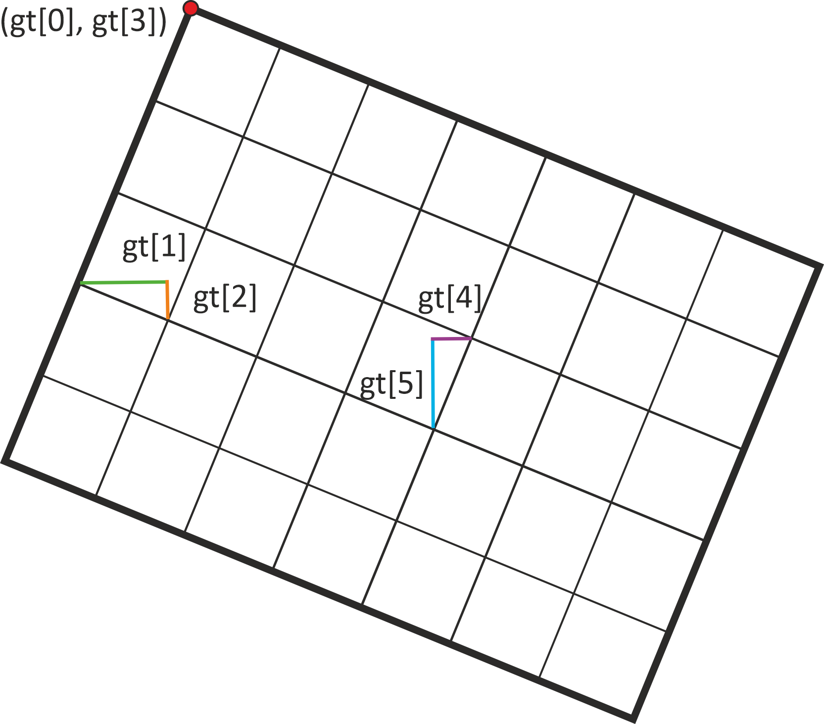
Performant access to geospatial raster data is a crutial task involving coordinate to pixel index transformations or georeferencing image data. Such a task is completely independent from the data values themselves, and can solely work with the six affine geotransformation parameters, a spatial reference system, and the dimentions of a raster image.
The geospatial representation of a raster image has been realised with the class RasterTile, which is available within the tile module of pytileproj.
Initialisation#
The constructor of RasterTile expects the following arguments:
n_rows: Number of rows or height in pixels of the rastern_cols: Number of columns or width in pixels of the rastercrs: A spatial reference system represented by anything pyproj supports, e.g., EPSG code, PROJ4 string, WKT string, …geotrans(optional): tuple containing the six GDAL affine geotransformation parametersname(optional): Name of the raster tilepx_origin(optional): The world system origin of the pixels (see Properties).
How the six geotransformation parameters relate to a georeferenced raster can be seen in the figure below.
from pytileproj import RasterTile

# initialisation of variables
n_rows = 50
n_cols = 50
epsg = 4326
geotrans = (
    5,
    0.2,
    0,
    50,
    0,
    -0.2,
)  # ul_x, x_pixel_size, x_rot, ul_y, y_rot, y_pixel_size
tilename = "Tile 1"
# additional, optional parameter is px_origin
raster_tile = RasterTile(
    n_rows=n_rows, n_cols=n_cols, crs=epsg, geotrans=geotrans, name=tilename
)
print(raster_tile)  # noqa: T201
RasterTile
----------
Name:
Tile 1
Shape:
(50, 50)
Projection:
+proj=longlat +datum=WGS84 +no_defs +type=crs
Geotransformation parameters:
(5.0, 0.2, 0.0, 50.0, 0.0, -0.2)
Pixel origin:
ul
This is not the only way to create a raster geometry. You can also initialise a raster geometry from a given extent,
extent = (5, 40, 15, 50)
RasterTile.from_extent(extent, epsg, 0.2, 0.2)
RasterTile(None)
from a given projected geometry,
import pyproj
from shapely.geometry import Polygon

from pytileproj import ProjGeom

polygon = Polygon([(5, 40), (5, 50), (15, 50), (15, 40), (5, 40)])
proj_geom = ProjGeom(geom=polygon, crs=pyproj.CRS.from_epsg(4326))

RasterTile.from_geometry(proj_geom, 0.2, 0.2, name=tilename)
RasterTile(Tile 1)
or from a JSON string:
json_str = """
{
    "crs": 4326,
    "n_rows": 50,
    "n_cols": 50,
    "geotrans": [
        5.0,
        0.2,
        0.0,
        50.0,
        0.0,
        -0.2
    ],
    "px_origin": "ul",
    "name": "Tile 1"
}
"""
raster_tile = RasterTile.from_json(json_str)
All options above result in the same raster tile object.
Properties#
Now having a raster tile instance ready, we can continue with inspecting the properties of this object. The shape of the tile is defined by its width
raster_tile.width
50
and its height.
raster_tile.height
50
Direct shape access is possible with (height, width)
raster_tile.shape
(50, 50)
The same can be done by using actual world system coordinates. The width is accessable through
raster_tile.x_size
np.float64(10.0)
and the height through
raster_tile.y_size
np.float64(10.0)
The sizes of each pixel can be easily retrieved via
raster_tile.x_pixel_size
np.float64(0.2)
and
raster_tile.y_pixel_size
np.float64(0.2)
A very important thing of the relationship between pixel and world system coordinates is the anchor point or pixel origin, i.e. to what point in the pixel the coordinate refers to. By default the GDAL definition is used, which states that the origin is in the upper-left corner of the upper-left pixel. But with a RasterTile instance, you also have the option to choose between all other corner points and the pixel center.
The aformentioned properties and the different possibilities for the pixel origin are illustrated in the graphic below.
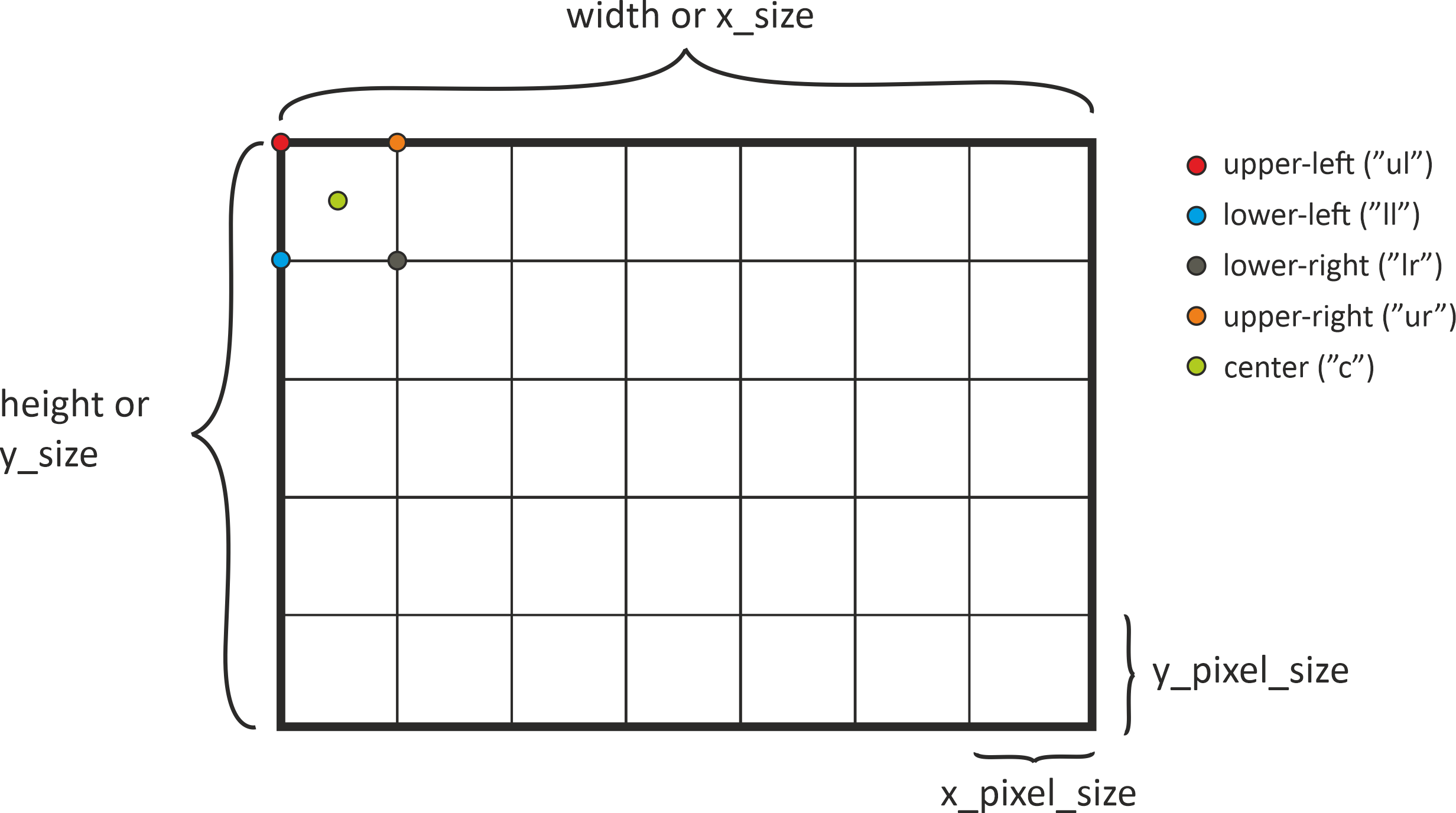
If you are interested in the corner points of the raster geometry, several properties help you to access the respective coordinates. For example, the lower-left corner, i.o.w. the first pixel in the last row, has the following coordinates:
raster_tile.ll_x, raster_tile.ll_y
(5.0, 40.2)
If you want to know the full coordinate extent (x_min, y_min, x_max, y_max), you can call
raster_tile.coord_extent
(5.0, 40.2, 14.8, 50.0)
Please note that all these coordinates refer to the pixel origin, which has been chosen during class initialisation. If you are interested in the full extent of the raster geometry (bold black line in the image before), you can use
raster_tile.outer_boundary_extent
(5.0, 40.0, 15.0, 50.0)
The corner points of the outer boundary are available via
raster_tile.outer_boundary_corners
((5.0, 40.0), (15.0, 40.0), (15.0, 50.0), (5.0, 50.0))
The full range of 1-D coordinates in a certain direction along the edges of a raster tile can be retrieved with
raster_tile.x_coords
array([ 5. ,  5.2,  5.4,  5.6,  5.8,  6. ,  6.2,  6.4,  6.6,  6.8,  7. ,
        7.2,  7.4,  7.6,  7.8,  8. ,  8.2,  8.4,  8.6,  8.8,  9. ,  9.2,
        9.4,  9.6,  9.8, 10. , 10.2, 10.4, 10.6, 10.8, 11. , 11.2, 11.4,
       11.6, 11.8, 12. , 12.2, 12.4, 12.6, 12.8, 13. , 13.2, 13.4, 13.6,
       13.8, 14. , 14.2, 14.4, 14.6, 14.8])
and
raster_tile.y_coords
array([50. , 49.8, 49.6, 49.4, 49.2, 49. , 48.8, 48.6, 48.4, 48.2, 48. ,
       47.8, 47.6, 47.4, 47.2, 47. , 46.8, 46.6, 46.4, 46.2, 46. , 45.8,
       45.6, 45.4, 45.2, 45. , 44.8, 44.6, 44.4, 44.2, 44. , 43.8, 43.6,
       43.4, 43.2, 43. , 42.8, 42.6, 42.4, 42.2, 42. , 41.8, 41.6, 41.4,
       41.2, 41. , 40.8, 40.6, 40.4, 40.2])
These coordinates only refer to the first row or first column. If you are interested in every coordinate contained within the raster geometry you can use:
raster_tile.xy_coords
(array([[ 5. ,  5. ,  5. , ...,  5. ,  5. ,  5. ],
        [ 5.2,  5.2,  5.2, ...,  5.2,  5.2,  5.2],
        [ 5.4,  5.4,  5.4, ...,  5.4,  5.4,  5.4],
        ...,
        [14.4, 14.4, 14.4, ..., 14.4, 14.4, 14.4],
        [14.6, 14.6, 14.6, ..., 14.6, 14.6, 14.6],
        [14.8, 14.8, 14.8, ..., 14.8, 14.8, 14.8]], shape=(50, 50)),
 array([[50. , 49.8, 49.6, ..., 40.6, 40.4, 40.2],
        [50. , 49.8, 49.6, ..., 40.6, 40.4, 40.2],
        [50. , 49.8, 49.6, ..., 40.6, 40.4, 40.2],
        ...,
        [50. , 49.8, 49.6, ..., 40.6, 40.4, 40.2],
        [50. , 49.8, 49.6, ..., 40.6, 40.4, 40.2],
        [50. , 49.8, 49.6, ..., 40.6, 40.4, 40.2]], shape=(50, 50)))
The boundary of the raster tile is also availabe on a higher-level, e.g. as a WKT string, OGR or shapely geometry.
raster_tile.boundary_wkt
'POLYGON ((5 40, 15 40, 15 50, 5 50, 5 40))'
Not all properties have been discussed here. Please take look at the API documentation to explore the full range of offered functionality.
Plotting#
A very nice feature of a raster tile is that you can plot it on a map. Several keywords can help you to beautify your plot. First, we can simply try to plot the raster tile we have created before.
import matplotlib.pyplot as plt

plt.figure(figsize=(15, 15))
_ = raster_tile.plot()
Since the full extent of the projection is chosen by default, we can try limit the extent with:
plt.figure(figsize=(12, 12))
_ = raster_tile.plot(extent=(0, 35, 20, 55))
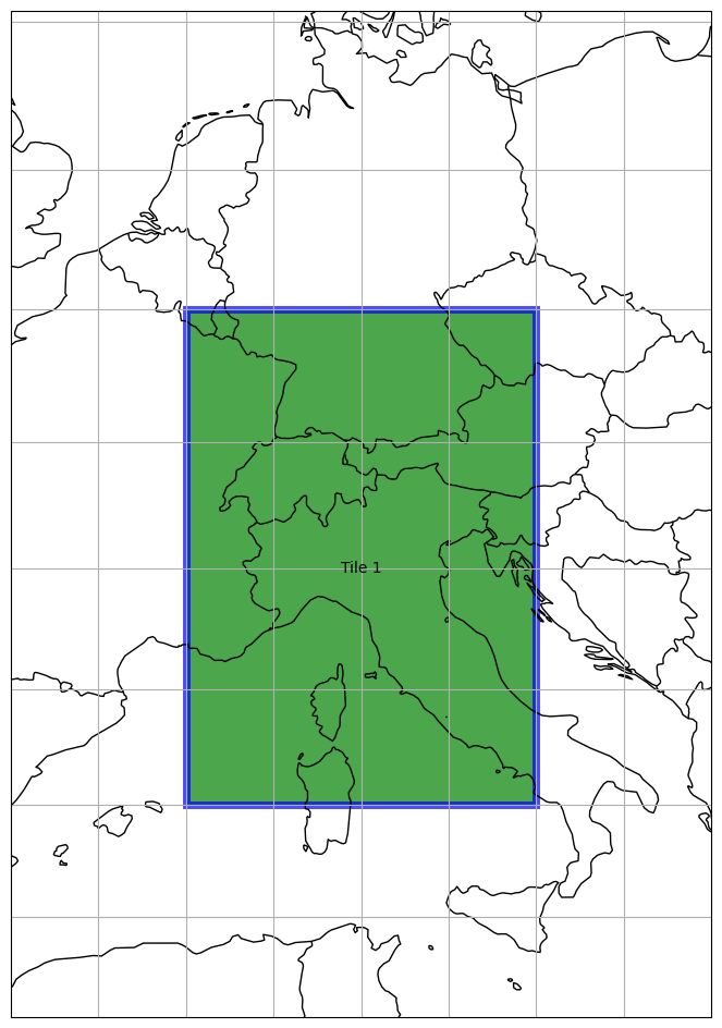
The plot function also allows to change the projection. We can try to define a new one, e.g. a Pseudo-Mercator projection, and use it for our new map.
plt.figure(figsize=(12, 12))
_ = raster_tile.plot(
    label_tile=True,
    facecolor="green",
    edgecolor="blue",
    edgewidth=5,
    alpha=0.7,
    proj=3857,
    extent=(0, 35, 20, 55),
)
Topological operations#
Raster tiles provide the functionality to interact with each other or with other geometries. The first set of functions checks for certain topological constrains, e.g. WITHIN, INTERSECTS, TOUCHES or OVERLAPS. To try this out we can create additional raster tiles.
geotrans_within = (6, 0.2, 0, 49, 0, -0.2)
raster_tile_within = RasterTile(
    n_rows=25, n_cols=25, crs=epsg, geotrans=geotrans_within, name="WITHIN"
)

geotrans_outer = (1, 0.2, 0, 49, 0, -0.2)
raster_tile_outer = RasterTile(
    n_rows=15, n_cols=5, crs=epsg, geotrans=geotrans_outer, name="OUTER"
)

geotrans_overlap = (12, 0.2, 0, 45, 0, -0.2)
raster_tile_overlap = RasterTile(
    n_rows=15, n_cols=30, crs=epsg, geotrans=geotrans_overlap, name="OVERLAPS"
)

geotrans_touch = (10, 0.2, 0, 40, 0, -0.2)
raster_tile_touch = RasterTile(
    n_rows=35, n_cols=25, crs=epsg, geotrans=geotrans_touch, name="TOUCHES"
)
plt.figure(figsize=(12, 12))
ax_1 = raster_tile.plot(extent=(0, 35, 20, 55))
_ = raster_tile_within.plot(
    ax=ax_1,
    label_tile=True,
    facecolor="blue",
    edgecolor="blue",
    edgewidth=2,
    alpha=0.7,
    extent=(0, 35, 20, 55),
)
_ = raster_tile_outer.plot(
    ax=ax_1,
    label_tile=True,
    facecolor="orange",
    edgecolor="orange",
    edgewidth=2,
    alpha=0.7,
    extent=(0, 35, 20, 55),
)
_ = raster_tile_overlap.plot(
    ax=ax_1,
    label_tile=True,
    facecolor="green",
    edgecolor="green",
    edgewidth=2,
    alpha=0.7,
    extent=(0, 35, 20, 55),
)
_ = raster_tile_touch.plot(
    ax=ax_1,
    label_tile=True,
    facecolor="purple",
    edgecolor="purple",
    edgewidth=2,
    alpha=0.7,
    extent=(0, 35, 20, 55),
)
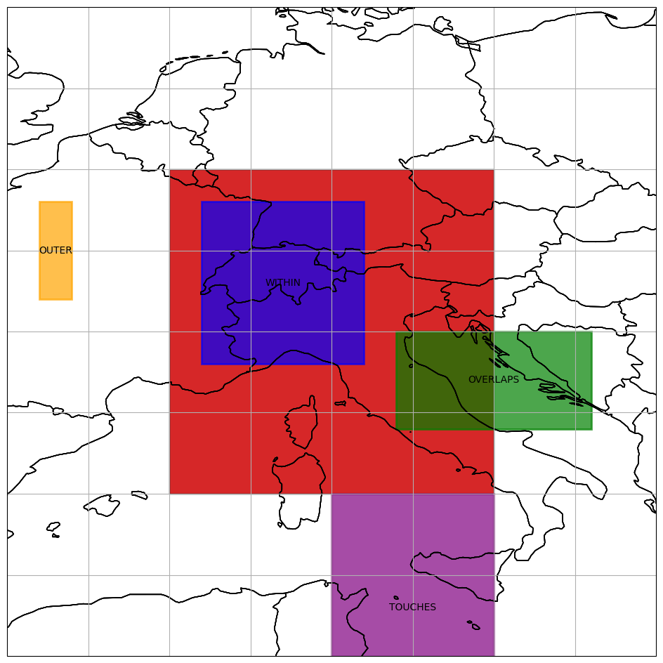
(
    raster_tile_within.within(raster_tile),
    raster_tile_within.intersects(raster_tile),
    raster_tile_within.touches(raster_tile),
    raster_tile_within.overlaps(raster_tile),
)
(True, True, False, False)
(
    raster_tile_outer.within(raster_tile),
    raster_tile_outer.intersects(raster_tile),
    raster_tile_outer.touches(raster_tile),
    raster_tile_outer.overlaps(raster_tile),
)
(False, False, False, False)
(
    raster_tile_overlap.within(raster_tile),
    raster_tile_overlap.intersects(raster_tile),
    raster_tile_overlap.touches(raster_tile),
    raster_tile_overlap.overlaps(raster_tile),
)
(False, True, False, True)
(
    raster_tile_touch.within(raster_tile),
    raster_tile_touch.intersects(raster_tile),
    raster_tile_touch.touches(raster_tile),
    raster_tile_touch.overlaps(raster_tile),
)
(False, True, True, False)
Coordinate conversions#
A raster tile also provides an interface for pixel to coordinate (rc2xy) and coordinate to pixel (xy2rc) conversions.
import numpy as np

rows, cols = np.meshgrid(np.arange(25, 30), np.arange(0, 25))
x_coords, y_coords = raster_tile.rc2xy(rows.flatten(), cols.flatten())
x_coords, y_coords
(array([5. , 5. , 5. , 5. , 5. , 5.2, 5.2, 5.2, 5.2, 5.2, 5.4, 5.4, 5.4,
        5.4, 5.4, 5.6, 5.6, 5.6, 5.6, 5.6, 5.8, 5.8, 5.8, 5.8, 5.8, 6. ,
        6. , 6. , 6. , 6. , 6.2, 6.2, 6.2, 6.2, 6.2, 6.4, 6.4, 6.4, 6.4,
        6.4, 6.6, 6.6, 6.6, 6.6, 6.6, 6.8, 6.8, 6.8, 6.8, 6.8, 7. , 7. ,
        7. , 7. , 7. , 7.2, 7.2, 7.2, 7.2, 7.2, 7.4, 7.4, 7.4, 7.4, 7.4,
        7.6, 7.6, 7.6, 7.6, 7.6, 7.8, 7.8, 7.8, 7.8, 7.8, 8. , 8. , 8. ,
        8. , 8. , 8.2, 8.2, 8.2, 8.2, 8.2, 8.4, 8.4, 8.4, 8.4, 8.4, 8.6,
        8.6, 8.6, 8.6, 8.6, 8.8, 8.8, 8.8, 8.8, 8.8, 9. , 9. , 9. , 9. ,
        9. , 9.2, 9.2, 9.2, 9.2, 9.2, 9.4, 9.4, 9.4, 9.4, 9.4, 9.6, 9.6,
        9.6, 9.6, 9.6, 9.8, 9.8, 9.8, 9.8, 9.8]),
 array([45. , 44.8, 44.6, 44.4, 44.2, 45. , 44.8, 44.6, 44.4, 44.2, 45. ,
        44.8, 44.6, 44.4, 44.2, 45. , 44.8, 44.6, 44.4, 44.2, 45. , 44.8,
        44.6, 44.4, 44.2, 45. , 44.8, 44.6, 44.4, 44.2, 45. , 44.8, 44.6,
        44.4, 44.2, 45. , 44.8, 44.6, 44.4, 44.2, 45. , 44.8, 44.6, 44.4,
        44.2, 45. , 44.8, 44.6, 44.4, 44.2, 45. , 44.8, 44.6, 44.4, 44.2,
        45. , 44.8, 44.6, 44.4, 44.2, 45. , 44.8, 44.6, 44.4, 44.2, 45. ,
        44.8, 44.6, 44.4, 44.2]))
rows, cols = raster_tile.xy2rc(x_coords, y_coords)
rows, cols
(array([25, 26, 27, 28, 29, 25, 26, 27, 28, 29, 25, 26, 27, 28, 29, 25, 26,
        27, 28, 29, 25, 26, 27, 28, 29, 25, 26, 27, 28, 29, 25, 26, 27, 28,
        29, 25, 26, 27, 28, 29, 25, 26, 27, 28, 29, 25, 26, 27, 28, 29, 25,
        26, 27, 28, 29, 25, 26, 27, 28, 29, 25, 26, 27, 28, 29, 25, 26, 27,
        28, 29, 25, 26, 27, 28, 29, 25, 26, 27, 28, 29, 25, 26, 27, 28, 29,
        25, 26, 27, 28, 29, 25, 26, 27, 28, 29, 25, 26, 27, 28, 29, 25, 26,
        27, 28, 29, 25, 26, 27, 28, 29, 25, 26, 27, 28, 29, 25, 26, 27, 28,
        29, 25, 26, 27, 28, 29]),
 array([ 0,  0,  0,  0,  0,  1,  1,  1,  1,  1,  2,  2,  2,  2,  2,  3,  3,
         3,  3,  3,  4,  4,  4,  4,  4,  5,  5,  5,  5,  5,  6,  6,  6,  6,
         6,  7,  7,  7,  7,  7,  8,  8,  8,  8,  8,  9,  9,  9,  9,  9, 10,
        10, 10, 10, 10, 11, 11, 11, 11, 11, 12, 12, 12, 12, 12, 13, 13, 13,
        13, 13, 14, 14, 14, 14, 14, 15, 15, 15, 15, 15, 16, 16, 16, 16, 16,
        17, 17, 17, 17, 17, 18, 18, 18, 18, 18, 19, 19, 19, 19, 19, 20, 20,
        20, 20, 20, 21, 21, 21, 21, 21, 22, 22, 22, 22, 22, 23, 23, 23, 23,
        23, 24, 24, 24, 24, 24]))
Magic methods#
For some of the aforementioned functions a set of magic methods are available to enable a Pythonic usage of a raster tile. This involves for instance the WITHIN check, which is internally called when using Pythons in.
raster_tile_within in raster_tile, raster_tile_outer in raster_tile
(True, False)
Two raster tiles are considered (spatially) the same if they have the same outer boundary corners, number of rows and number of cols.
raster_tile_eq = RasterTile(
    n_rows=n_rows, n_cols=n_cols, crs=epsg, geotrans=geotrans, name="Tile 2"
)

raster_tile == raster_tile_eq, raster_tile == raster_tile_overlap
(True, False)
The str method returns the WKT representation of the raster tile.
str(raster_tile)
'RasterTile \n---------- \nName: \nTile 1 \nShape: \n(50, 50)\nProjection: \n+proj=longlat +datum=WGS84 +no_defs +type=crs\nGeotransformation parameters: \n(5.0, 0.2, 0.0, 50.0, 0.0, -0.2)\nPixel origin: \nul'