Appendix C — Harmonic Parameters of Sentinel 1 Backscatter Time Series

In this notebook, we will show the concept of extracting coefficients that describe seasonal patterns in Sentinel 1 radar backscatter variability. Namely, sine and cosine functions as harmonic oscillators are used to describe periodicities in the time series of, either VV or VH polarisations, backscatter. Those can then be removed from time series and what is left would generally be the noise or transient events, for example floods, volcano erruptions, and whatever is possible to detect with radar Earth Observation data.

C.1 Prerequisites

Concepts	Importance	Notes
Intro to xarray	Necessary
Intro to Flood mapping	Necessary
Documentation hvPlot	Helpful	Interactive plotting

Time to learn: 10 min

C.2 Imports

import folium
import holoviews as hv
import hvplot.xarray  # noqa
import matplotlib.pyplot as plt
import numpy as np
import pandas as pd
import xarray as xr

Loading sigma nought time series.

timeseries_dc = xr.open_dataset(
    "simplecache::zip:///::https://huggingface.co/datasets/martinschobben/tutorials/resolve/main/harmonic-parameters.zarr.zip",  # noqa
    engine="zarr",
    storage_options={
        "simplecache": {"cache_storage": "/tmp/fsspec_cache/harmonic-parameters"}
    },
)
timeseries_dc

The data that is loaded represents VV and VH backsatter polarisations, as detected by Sentinel-1 radar instrument. The two points of interest are on Sicily, nearby Lentini and Catania.

latmin, latmax = 37.283606, 37.40621527385254
lonmin, lonmax = 14.826223, 15.109736519516783

bounding_box = [
    [latmin, lonmin],
    [latmax, lonmax],
]

map = folium.Map(
    location=[
        (latmin + latmax) / 2,
        (lonmin + lonmax) / 2,
    ],
    zoom_start=9,
    zoom_control=True,
    scrollWheelZoom=False,
    dragging=True,
)


folium.Rectangle(
    bounds=bounding_box,
    color="red",
).add_to(map)

folium.Marker(
    location=[37.37489461337563, 14.884886613876311],
    popup="Selected Pixel in the flooded land in 2018",
    icon=folium.Icon(color="red"),
).add_to(map)

folium.Marker(
    location=[37.32275297904196, 14.947068995810364],
    popup="Selected Pixel in lake Lentini",
    icon=folium.Icon(color="red"),
).add_to(map)

map

Make this Notebook Trusted to load map: File -> Trust Notebook

Let’s plot time series of those two points.

event_date = pd.to_datetime("2018-05-17")

lake_curve = timeseries_dc.sel(point="lake").VV.hvplot(
    label="Lake Lentini VV",
    width=800,
    height=300,
    color="navy",
    ylabel="Sigma0 VV (dB)",
    xlabel="Time",
    title="Lake Lentini Pixel",
)

land_curve = timeseries_dc.sel(point="land").VV.hvplot(
    label="Land Pixel VV",
    width=800,
    height=300,
    color="olive",
    ylabel="Sigma0 VV (dB)",
    xlabel="Time",
    title="Flooded Land Pixel",
)

event_line = hv.VLine(event_date).opts(color="red", line_dash="dashed", line_width=2)

lake_plot = lake_curve * event_line
land_plot = land_curve * event_line

(lake_plot + land_plot).cols(1)

C.3 The Concept of Harmonic Parameters

C.3.1 One Harmonic in Traditional Form

A single harmonic is an oscillatory function, which can be expressed as:

\[ f(t) = A \cos \left( \frac{2\pi}{n} t + \phi \right) \]

where: - $ A $ is the amplitude of the harmonic, - $ $ is the phase shift in radians, - $ n $ is the period in units of time, - $ 2/n $ angular frequency.

The amplitude here can represent a physical quantitiy of interest, for instance temperature, radar backscatter, soil moisture, etc. In a way, anything can be represented as signal and signal processing can be therefore applied to many different scientific fields.

# A simple harmonic oscillator

time = np.linspace(0, 300, 2000)
amplitude = 1.0
period = 20.0
phi = 0.0
y = amplitude * np.cos((2 * np.pi / period) * time + phi)

hv.Curve((time, y), "Time", "Amplitude").opts(
    title="Simple Cosine Plot", width=1000, height=600, line_width=2
)

Now, if we have measure a physical quantity over a long time period, for example temperature of some region, we have a time series. A harmonic regression is a least-square-fit of a harmonic function to the complex signal - or time series. In regard to microwave backscattering time series this property can be utilized to represent seasonal patterns caused by vegetation. This way we can filter out the vegetation signal from our microwave backscattering time series - to either better understand the physics behind this harmonic or to better detect events that don’t seasonally repeat, like flood events.

Harmonic parameters would be input parameters that define such fitted harmonic components, in this case: amplitude, shifting phase and period of an oscillating function. However, the period and starting phase are inside the non-linear (sinusoidal) function, so a linearisation has to be done, as those parameters are going to be estimated with a least-square regression algorithm. In our case we will only estimate phase shift and amplitude, not the period of the harmonics.

Using the angle sum identity:

\[ \cos(x + y) = \cos x \cos y - \sin x \sin y \]

we expand:

\[ A \cos \left( \frac{2\pi t}{n} + \phi \right) = A \left[ \cos \phi \cos \left( \frac{2\pi t}{n} \right) - \sin \phi \sin \left( \frac{2\pi t}{n} \right) \right] \]

C.3.1.1 Defining Coefficients $ c_i $ and $ s_i $

Now, we can define the coefficients, that have units of a physical quantity (amplitude, such as radar backscatter cross sections):

\[ c = A \cos \phi, \quad s = - A \sin \phi \]

so that the equation becomes:

\[ A \cos \left( \frac{2\pi t}{n} + \phi \right) = c \cdot \cos \left( \frac{2\pi t}{n} \right) + s \cdot \sin \left( \frac{2\pi t}{n} \right) \]

We can then extract the starting phase information outside of the sinusoidal function. The period information is still there, but only because in this case it is not estimated in least-square process, but predetermined.

C.3.1.2 Generalizing to $ k $ Harmonics

A complex signal is generally summation of many basic harmonic terms. Summing over all harmonics, we obtain:

\[ f(t) = f^0 + \sum_{i=1}^{k} \left[ c_i \cos \left( \frac{2\pi i t}{n} \right) + s_i \sin \left( \frac{2\pi i t}{n} \right) \right] \]

where:

$ f^0 $ is the mean function value,
$ c_i = A_i _i $ and $ s_i = - A_i _i $ are the harmonic coefficients.

In this form different periodicities are covered, for example with $ i = 1, 2, … k $, we can have periods of $ , $, and so on.

# Simulation of complex signal with many harmonics

t = np.linspace(0, 15, 1000)
k = 3

coefficients = [
    {"A": 3, "B": 2, "n": 2, "phi": 0},
    {"A": 1.5, "B": 0.5, "n": 5, "phi": np.pi / 4},
    {"A": 0.8, "B": 1.2, "n": 8, "phi": np.pi / 2},
]

colors = ["firebrick", "navy", "seagreen"]

harmonics = []
signal_sum = np.zeros_like(t)

for coeff in coefficients:
    harmonic = coeff["A"] * np.cos(
        (2 * np.pi * coeff["n"] * t) / 10 + coeff["phi"]
    ) + coeff["B"] * np.sin((2 * np.pi * coeff["n"] * t) / 10 + coeff["phi"])
    harmonics.append(harmonic)
    signal_sum += harmonic

max_amp = max(np.max(np.abs(h)) for h in harmonics + [signal_sum])

fig, axes = plt.subplots(k + 1, 1, figsize=(6, 8), sharex=True)

for i in range(k):
    axes[i].plot(t, harmonics[i], label=f"Harmonic {i + 1}", color=colors[i])
    axes[i].legend()
    axes[i].grid()
    axes[i].set_ylim(-max_amp, max_amp)

axes[k].plot(
    t,
    signal_sum,
    label="Summed Signal = Harmonic 1 + Harmonic 2 + Harmonic 3",
    color="black",
)
axes[k].legend()
axes[k].grid()
axes[k].set_xlabel("Time")
axes[k].set_ylim(-max_amp, max_amp)

plt.tight_layout()
plt.show()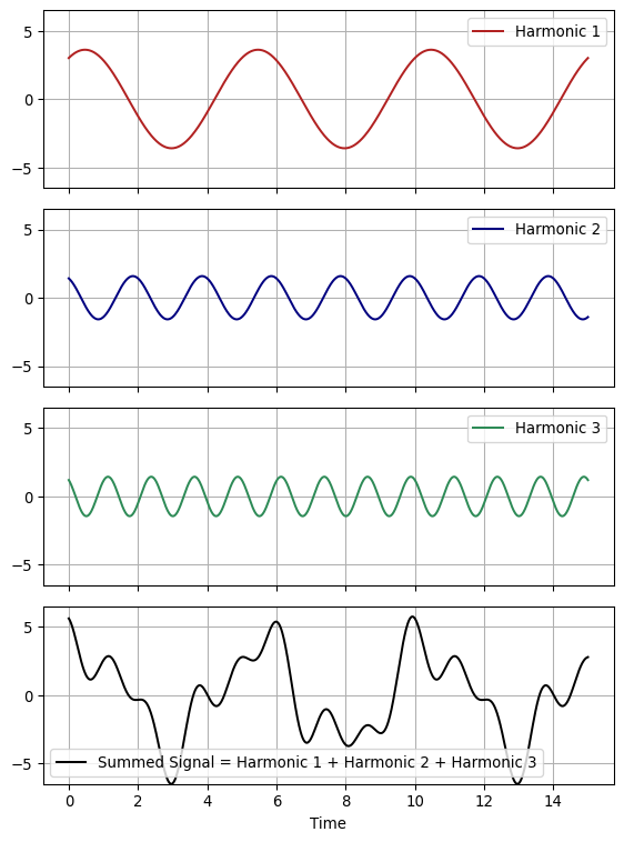

C.3.2 Recovering Amplitude and Phase

Now that we have estimated the harmonic coefficients $ c_i $** and **$ s_i $ wit the harmonic regression, we can recover the original amplitude and phase for a physical interpretation, as:

\[ A_i = \sqrt{c_i^2 + s_i^2} \]

\[ \phi_i = \tan^{-1} \left( -\frac{s_i}{c_i} \right) \]

C.3.3 Harmonic Model Equation for Radar Backscatter in Flood Detection Algorithm

The harmonic model function is given by:

\[ \widehat{\sigma}^0 (t_{doy}) = \sigma^0 + \sum_{i=1}^{k} \left\{ c_i \cos \left( \frac{2\pi i }{n} t_{doy} \right) + s_i \sin \left( \frac{2\pi i}{n} t_{doy} \right) \right\} \]

where:

\[ \sigma^0 &\quad \text{is the effective mean radar backscatter,} \\ \widehat{\sigma}^0 (t_{doy}) &\quad \text{is the estimated radar backscatter at time } t, \\ t_{doy} &\quad \text{is the time instance (as a day of a year),} \\ n &= 365 \text{ days} \\ c_i, s_i &\quad \text{are harmonic coefficients for } i = 1, 2, ..., k, \\ k &\quad \text{is the number of harmonic iterations}. \]

Let’s define a function that will fit a model like this with a least squares method, on a xarray array. Of course, the initial harmonic parameters first need to be estimated or known and their number depends on $k$.

def build_initial_parameters(array, k):
    """
    Constructs initial parameters and their names for harmonic curve fitting
    with option to choose number of k harmonics. Needed for
    xarray.DataArray.curvefit

    Parameters
    ----------
    array : xarray.DataArray
        The input 1D time series data for which the harmonic model is being
        fitted.

    k : int
        Number of harmonics to include in the model. For each harmonic, two
        parameters
        (cosine and sine coefficients) will be added: 'c1', 's1', ..., 'ck',
        'sk'.

    Returns
    -------
    param_names : list of str
        A list of parameter names in the order expected by the harmonic model
        function.
        Format: ['mean', 'c1', 's1', ..., 'ck', 'sk'].

    p0 : dict
        A dictionary containing initial guesses for each parameter.
        The mean is initialized from the data, and all harmonic coefficients are
        set to 1.0.
    """
    mean_val = float(array.mean().values)

    param_names = ["mean"]
    for i in range(1, k + 1):
        param_names += [f"c{i}", f"s{i}"]

    p0 = {"mean": mean_val}
    for name in param_names[1:]:
        p0[name] = 1.0

    return param_names, p0

def harmonic_model(t, mean, *coef):
    """
    Harmonic model function for fitting periodic components in time series data.
    To be passed in xarray.DataArray.curvefit as func argument

    This function computes a sum of sine and cosine terms up to a specified
    number of harmonics. The number of harmonics k is inferred from the length
    of the coef argument (must be 2 * k). The time variable t is expected to
    be in nanoseconds, e.g., from datetime64[ns] converted to int.

    Parameters
    ----------
    t : array-like or float
        Time values (in nanoseconds) over which to evaluate the harmonic model.
        This should match the time coordinate used in the original dataset,
        converted to integers via .astype('int64').

    mean : float
        The mean (baseline) value of the signal to which the harmonic components
        are added.

    *coef : float
        Variable-length list of harmonic coefficients, ordered as:
        [c1, s1, c2, s2, ..., ck, sk], where k = len(coef) // 2.
        Each `ci` and `si` corresponds to the cosine and sine coefficients for
        the i-th harmonic.

    Returns
    -------
    result : array-like or float
        The computed harmonic model values corresponding to the input t.

    Notes
    -----
    The fundamental frequency is assumed to be one cycle per year. The time
    normalization is based on the number of nanoseconds in a year (365 * 24 * 60
    * 60 * 1e9).
    """
    n = 365
    result = mean

    k = len(coef) // 2  # Number of harmonics

    for i in range(1, k + 1):
        c_i = coef[2 * (i - 1)]
        s_i = coef[2 * (i - 1) + 1]
        result += c_i * np.cos(2 * np.pi * i * t / n) + s_i * np.sin(
            2 * np.pi * i * t / n
        )

    return result

C.3.4 Harmonic Function Fitting

Now, the two time series can be selected and the coefficients can be estimated. We pick the VV polarisation for a land pixel and 3 harmonics (7 parameters).

land_VV_series = timeseries_dc.sel(point="land").VH
param_names, p0 = build_initial_parameters(land_VV_series, k=3)

fit_result = land_VV_series.curvefit(
    coords="time.dayofyear",
    func=harmonic_model,
    param_names=param_names,
    reduce_dims="time",
)

fit_result

Let’s extract and print estimated harmonic parameters for this pixel

estimated_params = fit_result.curvefit_coefficients.values

for name, val in zip(fit_result.param.values, estimated_params):
    print(f"{name: >6}: {val: .4f}")

  mean: -21.8654
    c1:  0.9572
    s1:  1.2286
    c2: -0.6606
    s2: -1.4352
    c3:  0.2654
    s3:  0.1653

Now, these coefficient can be used to construct a total harmonic signal.

# Extract estimated harmonic parameters and reconstruct a signal as xarray dataaray

mean = estimated_params[0]
coeffs = estimated_params[1:]

fitted_vals = harmonic_model(timeseries_dc["time.dayofyear"], mean, *coeffs)

fitted_da = xr.DataArray(
    fitted_vals, coords={"time": land_VV_series.time}, dims="time", name="Harmonic Fit"
)

# Plot the data

plot = land_VV_series.hvplot(
    label="Original", color="forestgreen", alpha=1
) * fitted_da.hvplot(label="Harmonic Fit", color="darkorange", line_width=2.5)

plot.opts(
    title="Harmonic Model Fit to VV Timeseries over Land",
    xlabel="Time",
    ylabel="VV backscatter",
    width=900,
    height=400,
)

We can see cycles that happen once a year, twice a year and three times a year, so it makes sense to work with time series over several years. Important parameter is a number of observations (NOBS) - the more observations the better. It directly relates to the uncertainty of our estimate. In this respect, the standard deviation is an important parameter, as it tells us how well our harmonic function fits the observations. It does not, however, tell us the uncertainty of the observations, just how well they align with seasonal patterns defined by the model.

residuals_land = land_VV_series - fitted_da
sse = np.sum(residuals_land.dropna(dim="time").values ** 2)

nobs = residuals_land.size
dof = nobs - (2 * k + 1)

stdev = np.sqrt(sse / dof)

print(f"Number of observations (NOBS): {nobs}")
print(f"Estimated standard deviation of the fit: {stdev: .4f}")

Number of observations (NOBS): 1214
Estimated standard deviation of the fit:  2.4799

Lets plot residuals that were used to calculate standard deviation and see the possible outliers that do not fit those seasonal patterns.

land_residuals_ts = residuals_land.dropna(dim="time")
land_residuals_ts.name = "Residual"

land_residuals_ts.hvplot(
    label="Residuals",
    color="firebrick",
    line_width=2,
    title="Residuals of Harmonic Fit (Land Pixel)",
    xlabel="Time",
    ylabel="Residual (VV)",
    width=900,
    height=300,
) * event_line

C.3.4.1 Lake Lentini Example

Lets see how time summed harmonic signal looks like for a lake pixel, where backscatter is more stable. Therefore, vegetation periodicities should be less pronounced over water.

lake_VV_series = timeseries_dc.sel(point="lake").VV
param_names_lake, p0_lake = build_initial_parameters(lake_VV_series, k=3)

fit_result = lake_VV_series.curvefit(
    coords="time", func=harmonic_model, p0=p0_lake, param_names=param_names_lake
)

estimated_params_lake = fit_result.curvefit_coefficients.values

for name, val in zip(fit_result.param.values, estimated_params_lake):
    print(f"{name: >6}: {val: .4f}")

  mean: -20.4635
    c1: -0.1479
    s1:  0.1429
    c2:  0.0382
    s2: -0.2207
    c3: -0.2902
    s3:  0.0870

mean = estimated_params_lake[0]
coeffs = estimated_params_lake[1:]

fitted_vals = harmonic_model(timeseries_dc["time.dayofyear"], mean, *coeffs)

fitted_da = xr.DataArray(
    fitted_vals, coords={"time": lake_VV_series.time}, dims="time", name="Harmonic Fit"
)

plot = lake_VV_series.hvplot(
    label="Original", color="navy", alpha=0.75
) * fitted_da.hvplot(label="Harmonic Fit", color="darkorange", line_width=2.5)

plot.opts(
    title="Harmonic Model Fit to VV Timeseries of a pixel inside lake Lentini",
    xlabel="Time",
    ylabel="VV backscatter",
    width=900,
    height=400,
)

residuals_lake = lake_VV_series - fitted_da
sse = np.sum(residuals_lake.dropna(dim="time").values ** 2)

nobs = residuals_lake.size
dof = nobs - (2 * k + 1)

stdev = np.sqrt(sse / dof)

print(f"Number of observations (NOBS): {nobs}")
print(f"Estimated standard deviation of the fit: {stdev: .4f}")

Number of observations (NOBS): 1214
Estimated standard deviation of the fit:  3.2212

lake_residuals_ts = residuals_lake.dropna(dim="time")
lake_residuals_ts.name = "Residual"

lake_residuals_ts.hvplot(
    label="Residuals",
    color="firebrick",
    line_width=2,
    title="Residuals of Harmonic Fit (Lake Pixel)",
    xlabel="Time",
    ylabel="Residual (VV)",
    width=900,
    height=300,
)

As one can notice, general pattern is a more stochastic signal. One can argue that setting k = 3 actually introduces artifacts, as the original signal was not periodic in the first place.

C.3.5 Overfitting Problem - Choosing $k$ iterations

Parameter $k$ that governs the number of harmonic terms, is usually two or three. Higher order terms would lead to overfitting. A flood event in time series would be an impulse (jump in backscatter value) that would propagate as an artefact if higher order harmonics are fitted to years-long time series. Higher order terms would usually have low amplitude, an estimation of those would highly depend on noise level in signal. Therefore, those harmonics would not be of a physical nature, or in other words, they wouldn’t represent seasonal vegetation cycles.

ks = [1, 2, 3, 10]
fitted_das = []

for k in ks:
    param_names, p0 = build_initial_parameters(land_VV_series, k)

    fit_result = land_VV_series.curvefit(
        coords="time.dayofyear",
        func=harmonic_model,
        param_names=param_names,
        reduce_dims="time",
    )

    estimated_params = fit_result.curvefit_coefficients.values
    mean = estimated_params[0]
    coeffs = estimated_params[1:]
    fitted_vals = harmonic_model(timeseries_dc["time.dayofyear"], mean, *coeffs)

    fitted_da = xr.DataArray(
        fitted_vals,
        coords={"time": land_VV_series.time},
        dims="time",
        name=f"Harmonic Fit (k={k})",
    )
    fitted_das.append(fitted_da)

plot = land_VV_series.hvplot(label="Original", color="black", alpha=0.6)

colors = ["red", "orange", "green", "blue"]

for da, k_val, color in zip(fitted_das, ks, colors):
    plot *= da.hvplot(label=f"k = {k_val}", line_width=2, color=color)

plot.opts(
    title="Harmonic Fits of VV Timeseries for Multiple k Values",
    xlabel="Time",
    ylabel="VV Backscatter",
    width=900,
    height=400,
    legend_position="top_left",
)