4 Dielectric Properties – JupyerHub Guide

In this notebook, we will investigate the varying backscatter values associated with different land surfaces like water bodies, forests, grasslands and urban areas. We will use backscatter data from the Sentinel-1 satellite and we will utilize the CORINE Land Cover dataset to classify and extrapolate these surfaces, enabling us to analyze how different land cover types influence backscatter responses.

import json

import holoviews as hv
import intake
import numpy as np
import rioxarray  # noqa: F401
import xarray as xr
from matplotlib.colors import BoundaryNorm, ListedColormap

from mrs.catalog import CorineColorCollection, get_intake_url
from mrs.plot import plot_corine_data, plot_variability_over_time

hv.extension("bokeh")

ⓘ

4.1 Load Sentinel-1 Data

For our analysis we are using sigma naught backscatering data from Sentinel-1. The images we are analyzing cover the region south of Vienna and west of Lake Neusiedl. We load the data and and apply again a preprocessing function. Here we extract the scaling factor and the date the image was taken from the metadata. We will focus our attention to a smaller area containing a part of the Lake Neusiedl Lake and its surrounding land. The obtainedxarray dataset and is then converted to an array, because we only have one variable, the VV backscatter values.

url = get_intake_url()
cat = intake.open_catalog(url)
sig0_da = cat.neusiedler.read().sig0.compute()

https://git.geo.tuwien.ac.at/public_projects/microwave-remote-sensing/-/raw/main/microwave-remote-sensing.yml

Let’s have a look at the data by plotting the first timeslice.

sig0_da.isel(time=0).plot(robust=True, cmap="Greys_r").axes.set_aspect("equal")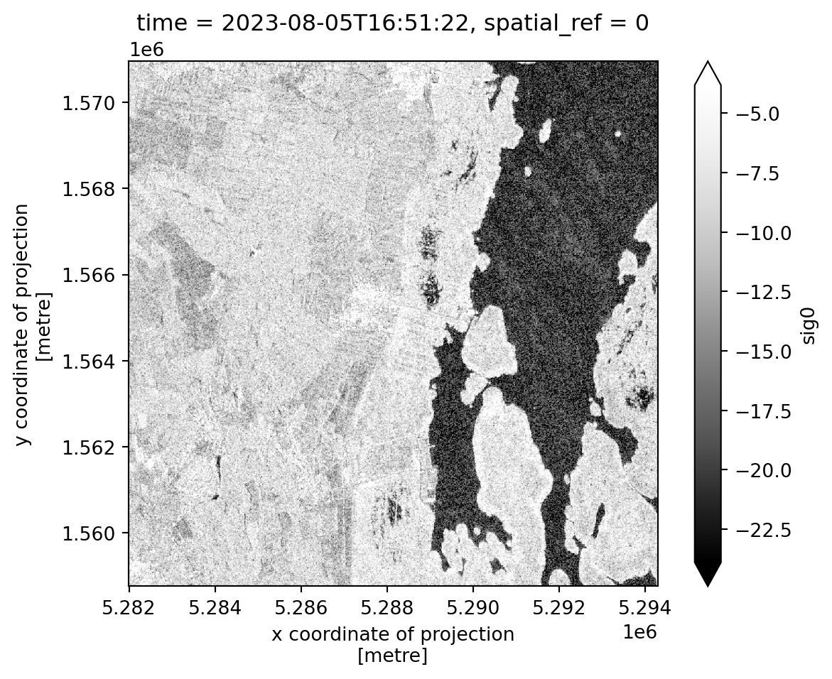

4.2 Load CORINE Landcover Data

We will load the CORINE Land Cover, which is a pan-European land cover and land use inventory with 44 thematic classes. The resolution of this classification is 100 by 100m and the file was created in 2018 (CORINE Land Cover).

cor_da = cat.corine.read().land_cover.compute()

4.2.1 Colormapping and Encoding

For the different land cover types we use the official color encoding which can be found in CORINE Land Cover.

# Load encoding and validate with Pydantic
with cat.corine_cmap.read()[0] as f:
    corine_colors = CorineColorCollection.model_validate(json.load(f))

# Create cmap and norm for plotting
colors = [info["color"].as_hex() for info in corine_colors.items]
categories = [info["value"] for info in corine_colors.items]
cmap = ListedColormap(colors)
norm = BoundaryNorm([*categories, max(categories) + 1], len(categories))

Now we can plot the CORINE Land Cover dataset.

present_landcover_codes = np.unique(cor_da.values[~np.isnan(cor_da.values)].astype(int))

# Create the plot
plot_corine_data(cor_da, cmap, norm, corine_colors, present_landcover_codes)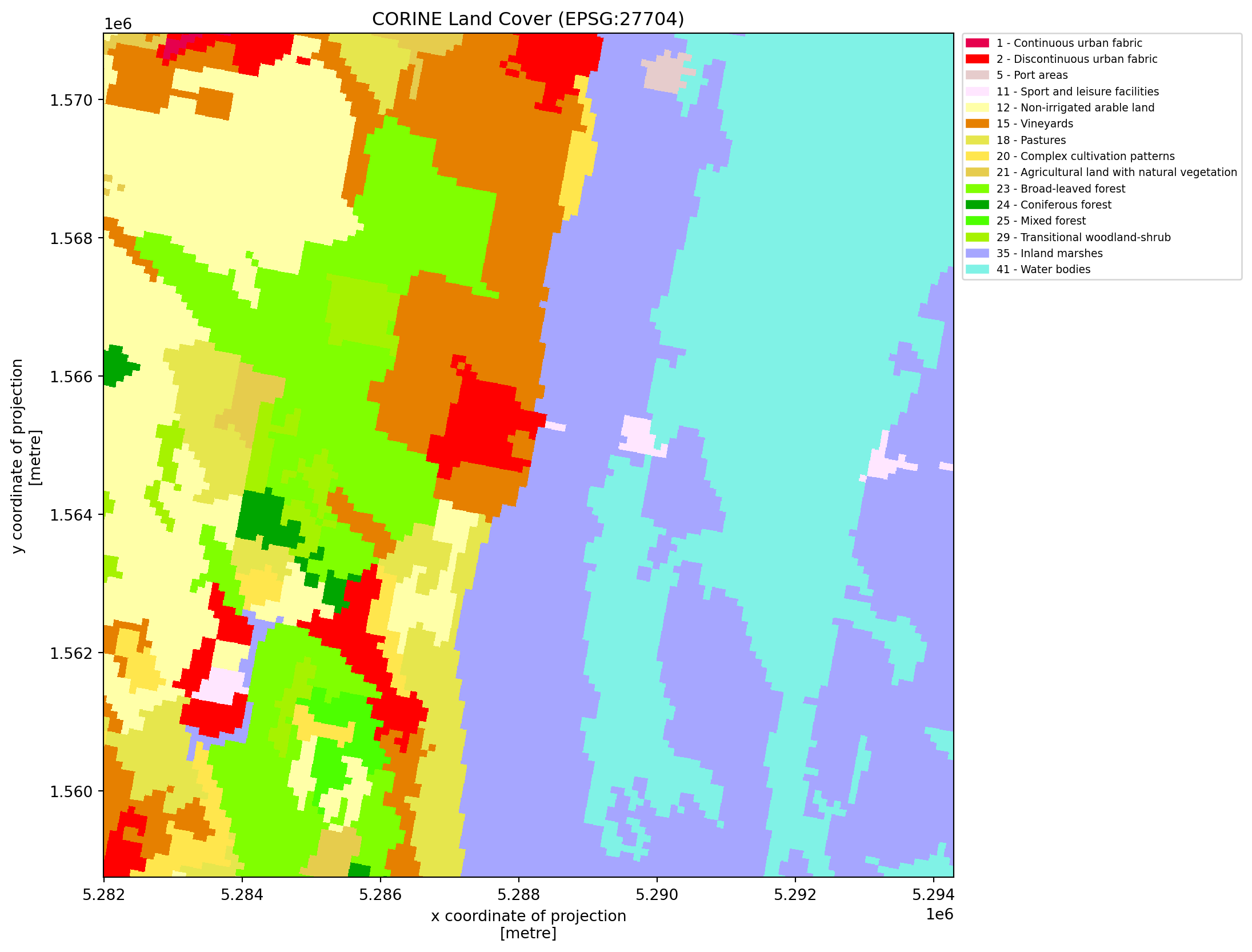

Now we are ready to merge the backscatter data (sig0_da) with the land cover dataset (cor_da) to have one dataset combining all data.

var_ds = xr.merge([sig0_da, cor_da]).drop_vars("band")
var_ds

/tmp/ipykernel_3059/125755716.py:1: FutureWarning: In a future version of xarray the default value for compat will change from compat='no_conflicts' to compat='override'. This is likely to lead to different results when combining overlapping variables with the same name. To opt in to new defaults and get rid of these warnings now use `set_options(use_new_combine_kwarg_defaults=True) or set compat explicitly.
  var_ds = xr.merge([sig0_da, cor_da]).drop_vars("band")

4.3 Backscatter Variability

With this combined dataset we can study backscatter variability in relation to natural media. For example we can look at the backscatter variability for water by clipping the dataset to only contain the land cover class water, like so:

# 41 = encoded value for water bodies
encoded_value_for_waterbodies = 41
waterbodies_mask = var_ds.land_cover == encoded_value_for_waterbodies
waterbodies_mask.plot().axes.set_aspect("equal")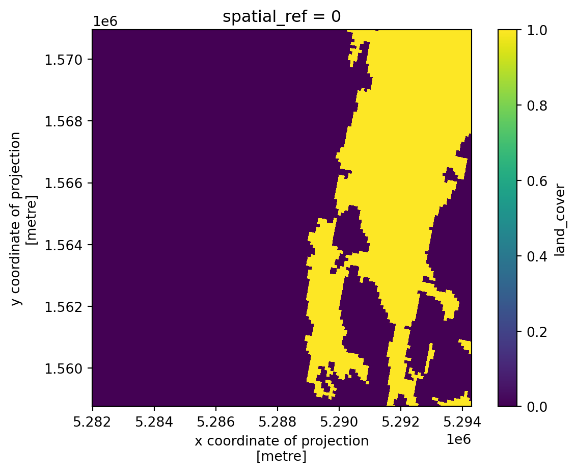

This gives use backscatter values over water only.

waterbodies_sig0 = var_ds.sig0.isel(time=0).where(waterbodies_mask)
waterbodies_sig0.plot(robust=True, cmap="Greys_r").axes.set_aspect("equal")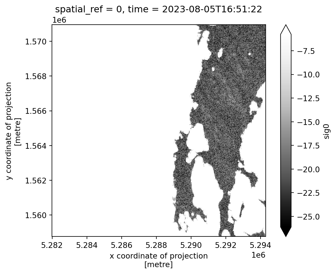

To get an idea of the variability we can create a histogram. Radar backscatter from water bodies fluctuates with surface roughness, which changes with wind conditions, creating spatial and temporal variations in signal intensity.

waterbodies_sig0.plot.hist(bins=50, edgecolor="black")

(array([5.0000e+00, 5.0000e+00, 8.0000e+00, 1.4000e+01, 3.5000e+01,
        7.8000e+01, 1.5600e+02, 3.0500e+02, 5.4000e+02, 1.0380e+03,
        1.9550e+03, 3.6850e+03, 6.9910e+03, 1.2269e+04, 1.9088e+04,
        2.6859e+04, 3.6217e+04, 4.5276e+04, 5.0939e+04, 4.9020e+04,
        3.9729e+04, 2.5400e+04, 1.2426e+04, 5.4390e+03, 2.6990e+03,
        2.0500e+03, 2.1330e+03, 2.6890e+03, 3.1490e+03, 3.9510e+03,
        4.2970e+03, 4.1110e+03, 3.6350e+03, 2.5900e+03, 1.6020e+03,
        7.5000e+02, 3.5200e+02, 1.2300e+02, 5.6000e+01, 3.7000e+01,
        2.8000e+01, 2.1000e+01, 1.3000e+01, 9.0000e+00, 1.0000e+01,
        8.0000e+00, 1.0000e+01, 5.0000e+00, 6.0000e+00, 4.0000e+00]),
 array([-37.91  , -36.9202, -35.9304, -34.9406, -33.9508, -32.961 ,
        -31.9712, -30.9814, -29.9916, -29.0018, -28.012 , -27.0222,
        -26.0324, -25.0426, -24.0528, -23.063 , -22.0732, -21.0834,
        -20.0936, -19.1038, -18.114 , -17.1242, -16.1344, -15.1446,
        -14.1548, -13.165 , -12.1752, -11.1854, -10.1956,  -9.2058,
         -8.216 ,  -7.2262,  -6.2364,  -5.2466,  -4.2568,  -3.267 ,
         -2.2772,  -1.2874,  -0.2976,   0.6922,   1.682 ,   2.6718,
          3.6616,   4.6514,   5.6412,   6.631 ,   7.6208,   8.6106,
          9.6004,  10.5902,  11.58  ]),
 <BarContainer object of 50 artists>)

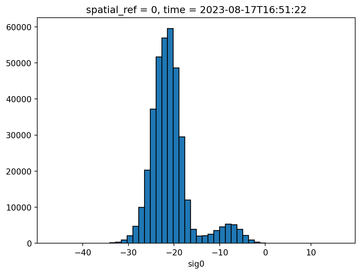
4.4 Variability over Time

Next we will look at the changes in variability in backscatter values over time for each of the CORINE Land Cover types. We do this by creating the following interactive plot. We can spot that backscatter in agricultural fields varies due to seasonal cycles like planting, growing, and harvesting, each of which changes vegetation structure. Changes in backscatter are strongly related to soil moisture content from irrigation or rainfall. Ultimately, phenological stages of crops and canopy moisture dynamics can affect the backscatter signal.

plot_variability_over_time(corine_colors.to_dict(), var_ds, present_landcover_codes)