The goal of this notebook is to read an interferogram image (i.e., 2-D array of phase values) and unwrap it. Phase unwrapping is a critical process in interferometry, which involves recovering unambiguous phase data from the interferogram.
A SAR interferogram represents the phase difference between two radar acquisitions (i.e., two SLC images). The phase difference is usually wrapped within a range of 0 to 2π, because the phase is inherently cyclical. When the true phase difference exceeds 2π, it gets “wrapped” into this range, creating a discontinuous phase signal. Phase unwrapping refers to the process of reconstructing the continuous phase field from the wrapped phase data.
Unwrapping an interferogram is essential for extracting correct information contained in the phase such as surface topography and earth surface deformations.
There are many approaches that tried to solve the unwrapping problem, tackling challenging scenarios involving noise or large phase discontinuities. Here we present the Network-flow Algorithm for phase unwrapping (C. W. Chen and H. A. Zebker, 2000), which is implemented in the snaphu package.
9.1 Loading Data
The data is stored on the Jupyterhub server, so we need to load it using their respective paths. In this notebook we will use the resulting wrapped interferogram from notebook “Interferograms”, but we need to process it in the radar geometry in order to unwrap it (while in notebook “Interferograms” we end the whole process by performing the geocoding, just for better visualization purposes).
from typing import Anyimport cmcrameri as cmc # noqa: F401import intakeimport numpy as npimport seaborn as snsimport snaphu # noqa: F401import xarray as xrfrom mrs.catalog import get_intake_urlfrom mrs.plot import ( plot_coarsened_image, plot_compare_coherence_mask_presence, plot_compare_wrapped_unwrapped_completewrapped, plot_different_coherence_thresholds, plot_displacement_map, plot_interferogram_map, plot_summary,)from mrs.processing import subsetting, unwrap_array
# Set cyclic and linear colormapscmap_cyc = sns.color_palette("hls", as_cmap=True)cmap_lin ="cmc.roma_r"cmap_disp ="cmc.vik"# Create a mask for the areas which have no datamask = ds.phase.where(ds.phase ==0, other=True, drop=False).astype(bool)
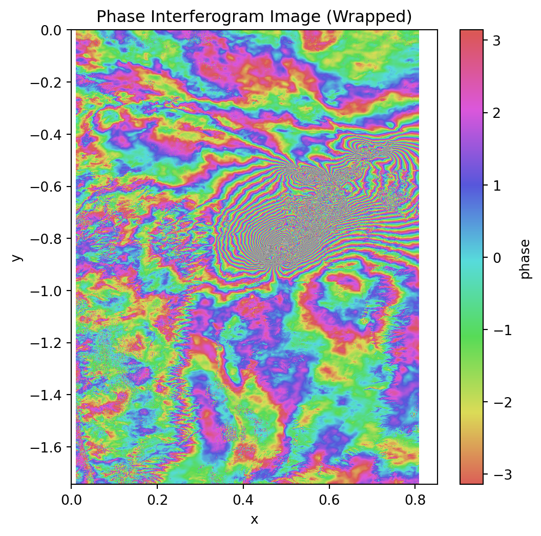
Let’s start by displaying the interferogram that needs to be unwrapped. Recall that due to the Slant Range geometry and the satellite acquisition pass (ascending, in our case), the image appears north/south flipped (with respect to the geocoded image)!
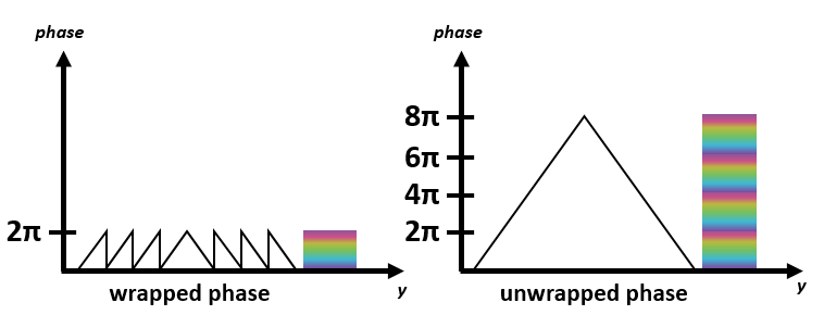
As we will be doing the unwrapping multiple times in this notebook let’s create a function that does the unwrapping for us on xarray DataArray objects. The actual core function where the unwrapping is happening is snaphu.unwrap_phase from the snaphu package. This function needs a 2D numpy array as input, where each pixel value is a complex number. Therefore, we have to convert the xarray DataArray to a 2D numpy array with complex values. We do that by combining the phase and intensity bands to a complex array. The actual unwrapping is essentially an addition of the phase values, such that the values are continuous and not between \(-\pi\) and \(\pi\).
Figure 1: Illustration of how the unwrapping of the phase works. (Source: ESA).
9.2.1 Unwrapping on a Subset
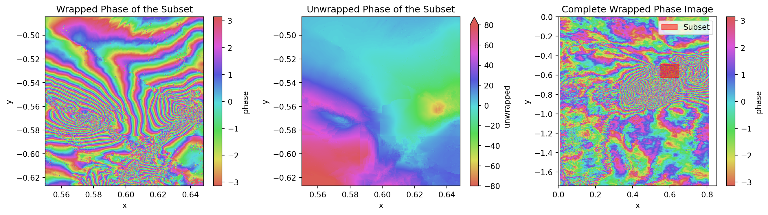
As the original image is too large to unwrap in a reasonable time, we will unwrap a subset of the image. In this case, we will unwrap an area of 500x500 pixels.
# Select a subset of the datadx, dy =500, 500x0, y0 =2800, 1700# Subsetting the data arrayssubset: xr.Dataset = subsetting(ds.where(mask), x0, y0, dx, dy)# Unwrap the subsetsubset = unwrap_array(subset, complex_var="cmplx", ouput_var="unwrapped")
Now let’s compare the wrapped and unwrapped phase images.
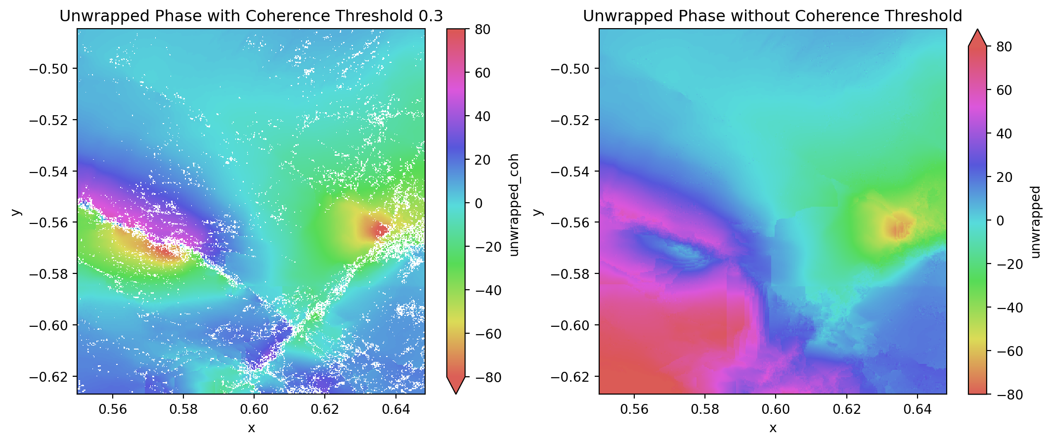
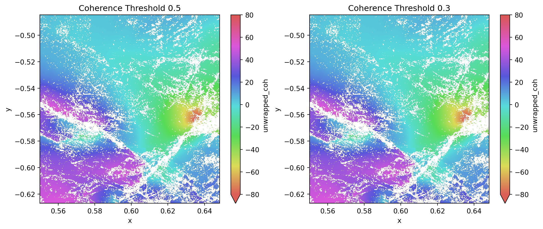
Additionally, can we try to calculate the unwrapped image by excluding pixels which the coherence values are lower than a certain threshold. This is done by masking the coherence image with the threshold value and then unwrapping the phase image with the masked coherence image.
A higher coherence threshold means that only pixels with a coherence value greater than 0.5 will be used for phase unwrapping. This would result in an unwrapping process that is likely more stable, with reduced noise (invalid phase information in the proximity of the earthquake faults is discarded). However, an excessive coherence threshold might have significant gaps or missing information, especially in areas where motion or surface changes have occurred. The choice of a coherence threshold depends on the balance you want to strike between the accuracy and coverage of the output unwrapped image.
Keep in mind that in case of large displacements, such as the Ridgecrest earthquake, phase unwrapping can be problematic and lead to poor results: when the displacement is large, the phase difference becomes wrapped multiple times, leading to phase aliasing. In this case, the phase values become ambiguous, we cannot distinguish between multiple phase wraps, thus leading to incorrect results.
9.3 Applying an Equation for the Displacement Map
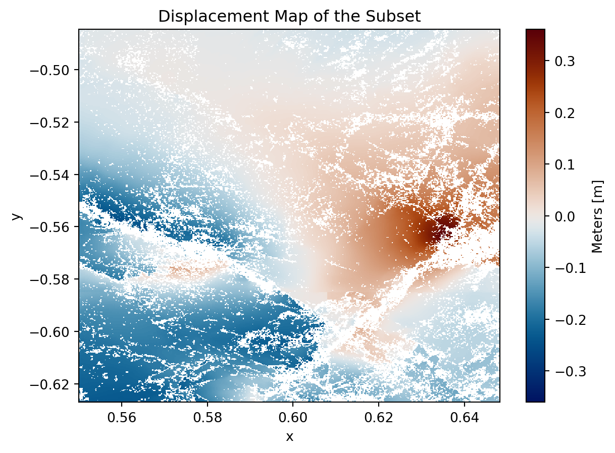
From the unwrapped phase image (we will use the phase masked with a coherence threshold of 0.3) we can calculate the displacement map using the following equation:
$ d = - _d $
where: - \(\lambda = 0.056\) for Sentinel-1 - \(\Delta \phi_d\) is the unwrapped image
This operation can be very useful for monitoring ground deformation.
def displacement(unw: xr.DataArray, lambda_val: float=0.056) -> xr.DataArray:"""Compute the displacement given the unwrapped phase."""return unw *-lambda_val / (4* np.pi)# Calculate the displacementdisp_subset = displacement(subset.unwrapped_coh)
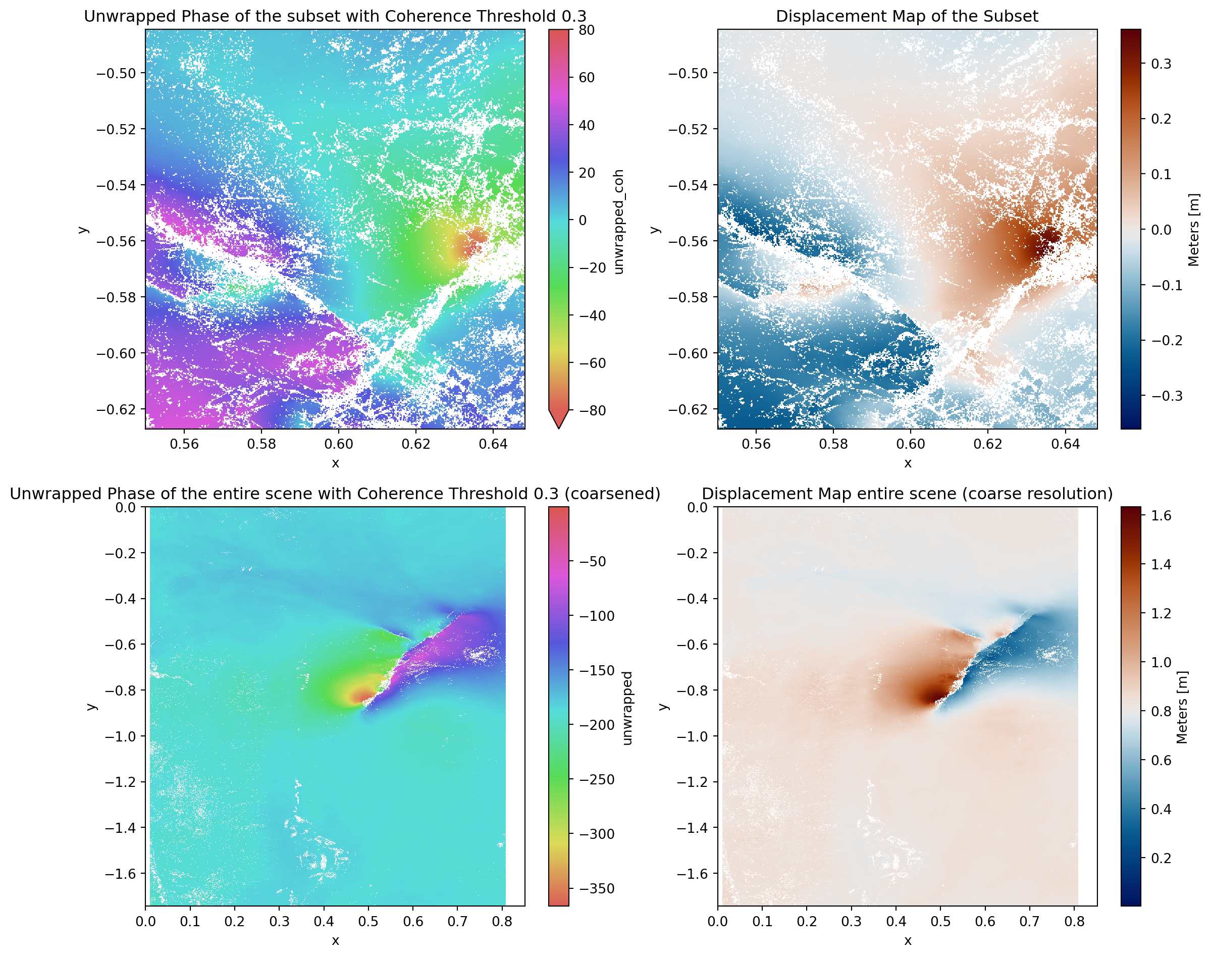
# Plot the displacement mapplot_displacement_map( subset=disp_subset, cmap_disp=cmap_disp, title="Displacement Map of the Subset",)
9.4 Coarsen Approach
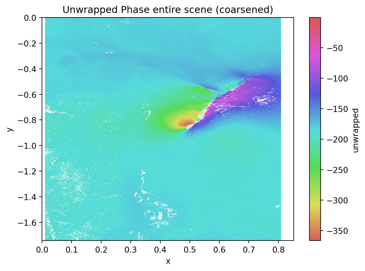
As the whole data is too large and the processing time already exceeds 20 minutes when using an image with 4000x4000 pixels, we can coarsen the image so that we can unwrap and compute the displacement for the whole scene.
We can now plot the unwrapped image of the low resolution image.
# Plot the unwrapped phaseplot_coarsened_image(lowres=lowres, cmap_cyc=cmap_cyc)
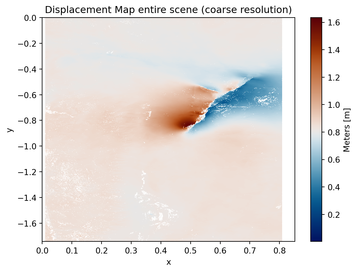
We can also now calculate the displacement map and compare them.
lowres_disp = displacement(lowres.unwrapped)# Plot the displacement mapplot_displacement_map( subset=lowres_disp, cmap_disp=cmap_disp, title="Displacement Map entire scene (coarse resolution)",)
Here is a summary of the previous plots: N.B.: The visualised deformation pattern is correct relative to radar geometry, but it will look “flipped” or “on the wrong side” when compared to a geocoded (map-aligned) image.


 Credits: NASA