11 Evaluating the Reliability of Remotely Sensed Soil Moisture

Comparing H SAF ASCAT Surface Soil Moisture with In-Situ Sensors

11.1 Overview

The aim of this notebook is to demonstrate and teach a workflow for validating ASCAT H SAF surface soil moisture (SSM) data, sampled at 6.25\(\,\)km distances, using in-situ sensors strategically placed in Mozambique. The evaluation in this context mainly assesses how well satellite-derived data aligns with the temporal patterns of in-situ soil water measurements. Remember, temporal dynamics are also crucial for anomaly detection in soil moisture records, which in turn affects our ability to monitor droughts (as discussed in the previous notebook). However, it is also a good practice to examine the absolute values of remotely sensed soil moisture. Such comprehensive validation processes are vital for forecasting, climate research, and decision-making, as they ensure the accuracy and reliability of weather data. By comparing different datasets, one can identify and address inconsistencies, thus enhancing the quality of meteorological records.

11.2 Imports

import folium
import hvplot
import hvplot.pandas
import pandas as pd

from envrs.download_path import make_url

11.3 In-situ Soil Moisture Sensors

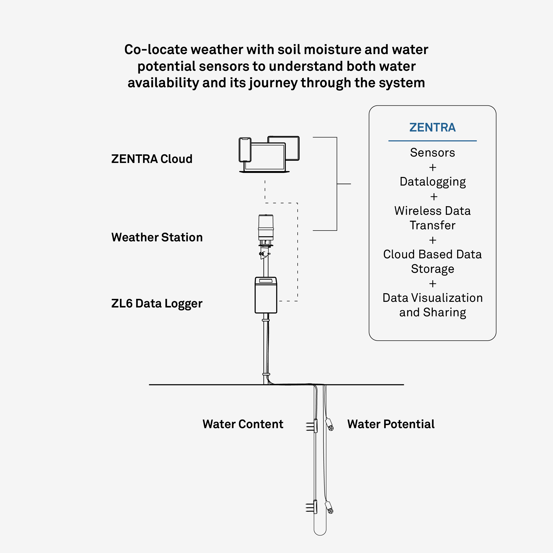
During the DrySat project we have placed 5 in-situ measuring stations (METER™, see image at the top) at strategic locations in Mozambique (Buzi, Chokwé, Mabalane, Mabote and Muanza). The locations are plotted on the following folium map for reference.

locations = {
    "Muanza": {"latitude": -18.9064758, "longitude": 34.7738921},
    "Chokwé": {"latitude": -24.5894393, "longitude": 33.0262595},
    "Mabote": {"latitude": -22.0530427, "longitude": 34.1227842},
    "Mabalane": {"latitude": -23.4258788, "longitude": 32.5448211},
    "Buzi": {"latitude": -19.9747305, "longitude": 34.1391065},
}


map = folium.Map(  # noqa: A001
    max_bounds=True,
    zoom_start=6,
    location=[-20, 34],
    scrollWheelZoom=False,
)

for i, j in locations.items():
    folium.Marker(
        location=[j["latitude"], j["longitude"]],
        popup=i,
    ).add_to(map)
map

Make this Notebook Trusted to load map: File -> Trust Notebook

These 5 stations each have 4 in-situ soil moisture sensors (Campbell Scientific™ HydroSense II with CS659) installed at depth intervals of 5, 10, 15, and 30\(\,\)cm. The deeper layers may not be directly pertinent to H SAF ASCAT SSM values, but they are important for another product derived from ASCAT data: the Soil Water Index, which assesses the moisture content of deeper layers. We will explore this further in a later notebook. The soil moisture content is measured every 15 minutes and directly stored in the cloud. Since their installation at the end of September 2023, these stations have continually gathered data. For this exercise, we have already cleaned and reformatted a portion of this dataset, which now includes only the measurements from the 5\(\,\)cm depth interval. Please consult us if you need access to the entire raw dataset.

It’s interesting to learn that the current in situ reference datasets are heavily focused on Europe and the USA (as seen on the ISMN MAP) due to data availability, which likely introduces bias into satellite products. Consequently, reference data from regions outside Europe and the USA are particularly valuable.

We load the data again as a pandas.DataFrame, like so:

RANGE = ("2023-09-30", "2025-05-06")
df_insitu = pd.read_csv(
    make_url("insitu_ssm_timeseries.csv"),
    index_col="time",
    parse_dates=True,
)
mask = (df_insitu.index > RANGE[0]) & (df_insitu.index <= RANGE[1])
df_insitu = df_insitu[mask]
df_insitu.head()

https://git.geo.tuwien.ac.at/api/v4/projects/1266/repository/files/insitu_ssm_timeseries.csv/raw?ref=main&lfs=true

	name	type	surface_soil_moisture	unit
time
2023-09-30 22:00:00	Buzi	in-situ	0.106400	m³/m³
2023-09-30 22:15:00	Buzi	in-situ	0.106434	m³/m³
2023-09-30 22:30:00	Buzi	in-situ	0.106400	m³/m³
2023-09-30 22:45:00	Buzi	in-situ	0.106434	m³/m³
2023-09-30 23:00:00	Buzi	in-situ	0.106400	m³/m³

Next, we will load the H SAF SSM 6.25\(\,\)km data as we did in the previous notebook. This time, however, we will filter the data to include only dates for which both ASCAT and in situ measurements are available.

df_ascat = pd.read_csv(
    make_url("ascat-6_25_ssm_timeseries.csv"),
    index_col="time",
    parse_dates=True,
)
mask = (df_ascat.index > RANGE[0]) & (df_ascat.index <= RANGE[1])
df_ascat = df_ascat[mask]
df_ascat.head()

https://git.geo.tuwien.ac.at/api/v4/projects/1266/repository/files/ascat-6_25_ssm_timeseries.csv/raw?ref=main&lfs=true

	name	type	surface_soil_moisture	unit
time
2023-09-30 19:16:05.482000384	Chokwé	ascat	54.48	%
2023-09-30 20:08:26.582000128	Chokwé	ascat	49.17	%
2023-10-01 06:29:06.317000192	Chokwé	ascat	54.97	%
2023-10-01 07:21:28.896999936	Chokwé	ascat	46.66	%
2023-10-01 18:55:21.116000256	Chokwé	ascat	53.92	%

Note, that the units of the in situ measurements differ when compared to the H SAF ASCAT SSM data. The in-situ sensors record soil moisture in volumetric units as cubic meters of water per cubic meters of soil [m\(^3\) / m\(^3\)]. By contrast, the satellite derived estimates are presented as the degree of saturation in the pore spaces of the remotely sensed soil.

11.4 Degree of Saturation vs. Volumetric Soil Water Content

To enable an absolute comparison of both data sources, we will first convert the degree of saturation used in the H SAF ASCAT dataset to volumetric units. This will allow us to compare the satellite-derived estimates with the measurements from the in-situ sensors. To achieve this, we need to know the porosity of the soil at the sensor locations. If the porosity is unknown, we can estimate it using a fixed particle density and the location-specific bulk density, as shown in the following expression.

\[ \text{Porosity} = 1 - \frac{\rho_{\text{bulk}}}{\rho_{\text{particle}}} \]

\[ \begin{aligned} \text{Porosity} &\quad \text{: Total pore space in the soil (-)} \\ \rho_{\text{bulk}} &\quad \text{: Bulk density (in g/cm³)} \\ \rho_{\text{particle}} &\quad \text{: Particle density (in g/cm³)} \\ \end{aligned} \]

For your convenience, we have obtain the location-specific bulk density for our targeted areas in Mozambique from SoilGrids. The particle density is typically averaged at about 2.65 g/cm³¹.

density_df = pd.DataFrame(
    {
        "name": ["Buzi", "Chokwé", "Mabalane", "Mabote", "Muanza"],
        "bulk_density": [1.25, 1.4, 1.4, 1.35, 1.25],
    }
).set_index("name")
density_df

	bulk_density
name
Buzi	1.25
Chokwé	1.40
Mabalane	1.40
Mabote	1.35
Muanza	1.25

We can now calculate the soil porosity from the bulk and particle density using the pandas transform method. After that, we will rename the column to “porosity”.

def calc_porosity(x: pd.Series) -> pd.Series:
    """Calculate Porosity.

    Parameters
    ----------
    x: Pandas.Series
        Bulk Density

    Returns
    -------
        Pandas.Series: Porosity

    """
    return 1 - x / 2.65


porosity_df = density_df.transform(calc_porosity).rename(
    columns={"bulk_density": "porosity"}
)
porosity_df

	porosity
name
Buzi	0.528302
Chokwé	0.471698
Mabalane	0.471698
Mabote	0.490566
Muanza	0.528302

Now we have the necessary information to convert the H SAF ASCAT SSM to volumetric units by using the following equation.

\[ \text{SSM}_{\text{abs}} = \text{Porosity} \cdot \frac{\text{SSM}_{\text{rel}}}{100} \]

\[ \begin{aligned} \text{SSM}_{\text{abs}} &\quad \text{: Absolute soil moisture, how much of the total soil volume is water (in m³/m³)} \\ \text{SSM}_{\text{rel}} &\quad \text{: Relative soil moisture in the pore spaces (in \%)} \end{aligned} \]

To apply this conversion to the HSAF dataset, we will first join the porosity values to the Soil Moisture (SSM) values based on the location names using a method called a “left join”. A left join in pandas merges two DataFrames while keeping all rows from the left DataFrame and adding matching rows from the right DataFrame. If there’s no match, it fills with NaN (see the figure for a schematic overview).

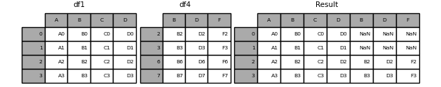
In this case, we’ll use the merge method, joining the left dataset on its ‘name’ column with the right dataset using its index labeled ‘name’.

df_ascat_porosity = df_ascat.merge(porosity_df, left_on="name", right_index=True)
df_ascat_porosity.head()

	name	type	surface_soil_moisture	unit	porosity
time
2023-09-30 19:16:05.482000384	Chokwé	ascat	54.48	%	0.471698
2023-09-30 20:08:26.582000128	Chokwé	ascat	49.17	%	0.471698
2023-10-01 06:29:06.317000192	Chokwé	ascat	54.97	%	0.471698
2023-10-01 07:21:28.896999936	Chokwé	ascat	46.66	%	0.471698
2023-10-01 18:55:21.116000256	Chokwé	ascat	53.92	%	0.471698

We can now use the pandas apply method to convert the units. This method takes the whole DataFrame as input allowing us to compute on two columns, while returning one column as output.

def deg2vol(df: pd.DataFrame) -> pd.Series:
    """Degree of Saturation to Volumetric Units.

    Parameters
    ----------
    df: Pandas.DataFrame
        Degree of Saturation

    Returns
    -------
        Pandas.Series: Volumetric Units

    """
    return df["porosity"] * df["surface_soil_moisture"] / 100


df_ascat_vol = df_ascat.copy()
df_ascat_vol["unit"] = "m³/m³"
df_ascat_vol["surface_soil_moisture"] = df_ascat_porosity.apply(deg2vol, axis=1)
df_ascat_vol.head()

	name	type	surface_soil_moisture	unit
time
2023-09-30 19:16:05.482000384	Chokwé	ascat	0.256981	m³/m³
2023-09-30 20:08:26.582000128	Chokwé	ascat	0.231934	m³/m³
2023-10-01 06:29:06.317000192	Chokwé	ascat	0.259292	m³/m³
2023-10-01 07:21:28.896999936	Chokwé	ascat	0.220094	m³/m³
2023-10-01 18:55:21.116000256	Chokwé	ascat	0.254340	m³/m³

11.5 Validation by Visual Inspection

The first step is to visually compare the time series. Visual inspection is essential for ensuring the validity and reliability of your results. It helps identify patterns and trends that might not be evident from data tables. Additionally, it is crucial for detecting outliers, which could indicate sensor malfunctions or data entry errors. In our case, we aim to see if both the in-situ and H SAF ASCAT SSM accurately reflect the characteristic seasonal rains of Mozambique.

To facilitate a clear overview, we will first concatenate the two datasets as follows:

df_combined = pd.concat([df_insitu, df_ascat_vol])
df_combined.head()

	name	type	surface_soil_moisture	unit
time
2023-09-30 22:00:00	Buzi	in-situ	0.106400	m³/m³
2023-09-30 22:15:00	Buzi	in-situ	0.106434	m³/m³
2023-09-30 22:30:00	Buzi	in-situ	0.106400	m³/m³
2023-09-30 22:45:00	Buzi	in-situ	0.106434	m³/m³
2023-09-30 23:00:00	Buzi	in-situ	0.106400	m³/m³

Next, we will use the hvplot extension for pandas to create interactive scatter plots for the time series.

df_combined.hvplot.scatter(
    x="time",
    y="surface_soil_moisture",
    by="type",
    groupby="name",
    frame_width=800,
    padding=(0.01, 0.1),
    alpha=0.5,
)

These plots already assure us that the trends in both data records align with the monotonic trends characteristic of soil wetting during Mozambique’s rainy season.

11.6 Quantitative Validation Metrics

We can now move to a more quantitative estimate. Correlation analysis is a valuable tool for validating meteorological records by comparing different datasets to ensure consistency and accuracy. It measures the strength and direction of the relationship between two variables. In the context of meteorological records, it helps assess how well different datasets align with each other in terms of temporal dynamics, serving as a quality assurance measure.

Before applying correlation analysis, we need to reshape our DataFrame by pairing the data to the same timestamps for each of the five locations. For this, we will use the groupby method in combination with the resample method. The resample method will adjust the time index to a new frequency of 1 day, using the median value to down sample the frequencies from 15 minutes to daily for both ASCAT and in-situ sensor data.

df_insitu_daily = (
    df_insitu.groupby("name")["surface_soil_moisture"]
    .resample("D")
    .median()
    .to_frame("in-situ")
)

df_ascat_vol_daily = (
    df_ascat_vol.groupby("name")["surface_soil_moisture"]
    .resample("D")
    .median()
    .to_frame("ascat")
)

df_resampled = df_ascat_vol_daily.join(df_insitu_daily)
df_resampled = df_resampled.dropna()
df_resampled.head()

		ascat	in-situ
name	time
Buzi	2023-10-01	0.068072	0.110634
	2023-10-03	0.048498	0.113430
	2023-10-05	0.067623	0.113479
	2023-10-06	0.052117	0.113479
	2023-10-08	0.060834	0.112111

The data is now ready for correlation analysis. For time series analysis, if you’re looking at trends and expect a linear relationship, Pearson correlation is straightforward and precise method.

\[ r = \frac{ \sum_{i=1}^{n} (x_i - \bar{x}) (y_i - \bar{y}) }{ \sqrt{ \sum_{i=1}^{n} (x_i - \bar{x})^2 } \sqrt{ \sum_{i=1}^{n} (y_i - \bar{y})^2 } } \]

where:

\[ \begin{aligned} n &\quad \text{: number of data points} \\ x_i \; \text{and} \; y_i &\quad \text{: individual sample points} \\ \bar{x} &\quad \text{: mean of the} \; x \; \text{values} \\ \bar{y} &\quad \text{: mean of the} \; y \; \text{values} \end{aligned} \]

The Pearson correlation coefficient ranges from -1 to 1:

\(r = 1\) indicates a perfect positive linear relationship.
\(r = -1\) indicates a perfect negative linear relationship.
\(r = 0\) indicates no linear relationship.

We implement this with pandas, as follows:

df_resampled.groupby("name").corr(method="pearson")

		ascat	in-situ
name
Buzi	ascat	1.000000	0.663829
Buzi	in-situ	0.663829	1.000000
Chokwé	ascat	1.000000	0.644887
Chokwé	in-situ	0.644887	1.000000
Mabalane	ascat	1.000000	0.729945
Mabalane	in-situ	0.729945	1.000000
Mabote	ascat	1.000000	0.584710
Mabote	in-situ	0.584710	1.000000
Muanza	ascat	1.000000	0.669616
Muanza	in-situ	0.669616	1.000000

Use Spearman correlation when the relationship between your time series is not necessarily linear but generally moves in the same direction (monotonic).

\[\rho = 1 - \frac{6 \sum d_i^2}{n(n^2 - 1)} \]

where:

\[ \begin{aligned} n &\quad \text{: number of observations} \\ d_i &\quad \text{: difference between the ranks of corresponding values} \; x_i \; \text{and} \; y_i \end{aligned} \]

The interpretation of \(\rho\) is the same as for the Pearson’s correlation (\(r\)) coefficient. Spearman is great for data where the ranking of values is important and is less affected by outliers and non-normal distributions. This makes it a robust choice for various types of data. It’s also easy to interpret because it focuses on the overall trend.

df_resampled.groupby("name").corr(method="spearman")

		ascat	in-situ
name
Buzi	ascat	1.000000	0.652317
Buzi	in-situ	0.652317	1.000000
Chokwé	ascat	1.000000	0.595828
Chokwé	in-situ	0.595828	1.000000
Mabalane	ascat	1.000000	0.754692
Mabalane	in-situ	0.754692	1.000000
Mabote	ascat	1.000000	0.720681
Mabote	in-situ	0.720681	1.000000
Muanza	ascat	1.000000	0.593781
Muanza	in-situ	0.593781	1.000000

The correlation coefficients for both Pearson and Spearman methods range between 0.6 and 0.8 across different locations, indicating moderate to high positive correlations between the ASCAT HSAF 6.25\(\,\)km data and the in-situ soil moisture estimates.

So far, we have only evaluated relative temporal trends in the two data sources. However, it is clear from the visual comparison of HSAF ASCAT SSM and in situ soil moisture that there are also absolute differences. To quantify these differences, we will first calculate the bias between in situ and remotely sensed soil moisture. Using Pandas, this involves comparing the mean of the target values (remotely sensed SSM) to the mean of the reference values (in situ SSM). Bias is determined by the difference between these means.

\[ \text{Bias} = \bar{x}_i - \bar{y}_i \]

where:

\[ \begin{aligned} \bar{y}_i &\quad \text{: mean target value (remotely sensed SSM)} \\ \bar{x}_i &\quad \text{: mean reference value (in situ SSM)} \end{aligned} \]

Which we can easily implement, like so:

(
    df_resampled.groupby("name")["in-situ"].mean()
    - df_resampled.groupby("name")["ascat"].mean()
)

name
Buzi        0.001074
Chokwé      0.012045
Mabalane   -0.061894
Mabote     -0.071499
Muanza     -0.040774
dtype: float64

Above, we observe the systematic error (in m\(^3\)/m\(^3\)) for each location. The H SAF ASCAT values are generally lower than the paired in situ observations, with the exception of Chokwé and Buzi. However, these differences are relatively small.

An interrelated yet distinct statistic is the Root Mean Square Error (RMSE).

\[ \text{RMSE} = \sqrt{\frac{1}{n} \sum_{i=1}^{n} (y_i - x_i)^2 } \]

where:

\[ \begin{aligned} n &\quad \text{: number of observations} \\ y_i &\quad \text{: target value (remotely sensed SSM)} \\ x_i &\quad \text{: reference value (in situ SSM)} \end{aligned} \]

Whereas bias contributes to the overall error measured by RMSE, RMSE captures both the bias and the variance components of the error. The relationship can be expressed through the bias-variance tradeoff:

Bias: Reflects the absolute difference among in situ and remotely sensed soil moisture
Variance: Reflects the relative differences among in situ and remotely sensed soil moisture
Irreducible Error: The inherent noise or randomness in the data that cannot be explained

The total error, as captured by RMSE, can be broken down as:

\[ \text{Total Error (RMSE)} = \text{Bias}^2+\text{Variance}+\text{Irreducible Error} \]

This can be implemented, as follows:

def rmse(df: pd.DataFrame) -> pd.Series:
    """Root Mean Square Error.

    Parameters
    ----------
    df: Pandas.DataFrame
        Target "ascat" and reference "in situ" columns

    Returns
    -------
        Pandas.Series: Root Mean Square Error

    """
    return ((df["ascat"] - df["in-situ"]) ** 2).mean() ** 0.5


df_resampled.groupby("name").apply(rmse)

name
Buzi        0.066416
Chokwé      0.071972
Mabalane    0.074553
Mabote      0.082575
Muanza      0.060688
dtype: float64

Here, we see that the RMSE ranges between 0.06 and 0.08 [m\(^3\) / m\(^3\)], which is small compared to the total range of H SAF ASCAT SSM. As a final step, we can visualize the relation of target (remotely sensed SSM) and reference values (in situ soil moisture) using hvplot.

hvplot.scatter_matrix(df_resampled.reset_index(level=0), c="name", alpha=0.3).opts(
    plot_size=300
)

Here, we observe that the relationship between in-situ and remotely sensed values is not entirely linear. Additionally, it indicates that soil moisture data is generally not normally distributed.

11.7 Scale of Measurement

We can only speculate about the reasons for the absolute and relative discrepancies, but it is important to note that the scale of in-situ measurements, which cover several centimeters around the device, compared to the averaged soil moisture value obtained by ASCAT, which encompasses about 50\(\,\)km\(^2\), might be a significant factor in explaining these differences. One can wonder what an averaged signal over such a broad area encompasses, as it can include a range of geomorphological, hydrological, and geological settings. Additionally, weather patterns can be confined to scales smaller than this area.

Rühlmann, M. Körschens, and J. Graefe, A new approach to calculate the particle density of soils considering properties of the soil organic matter and the mineral matrix, Geoderma, vol. 130, no. 3, pp. 272-283, Feb. 2006, doi: 10.1016/j.geoderma.2005.01.024.↩︎