12 Evaluating the Reliability of Remotely Sensed Droughts

Comparing Various Drought Indicators

12.1 Overview

This notebook continues the evaluation of drought indicators introduced in notebook 1. The H SAF ASCAT sensors onboard the MetOp series of polar-orbiting satellites supply near real-time surface soil moisture (SSM) estimates, with data extending back to 2007. This extensive record allows us to compute temporal anomalies from the SSM data, using the long-term mean as a baseline. These anomalies are then standardized as deviations, or Z scores.

As noted in notebook 1, ASCAT SSM is measured in degrees of saturation, making spatial patterns reliant on soil characteristics such as porosity. However, the temporal changes used for drought anomaly detection with Z scores can provide insights into spatial patterns of drought conditions without requiring auxiliary soil data.

We will leverage this feature to compare the H SAF ASCAT SSM-based drought indicators with other drought indicators, notably the Standardized Precipitation-Evapotranspiration Index ¹.

12.2 Imports

import cartopy.crs as ccrs
import datashader as ds
import holoviews as hv
import hvplot.pandas  # noqa
import numpy as np
import pandas as pd

from envrs.download_path import make_url

12.3 Standardized Precipitation-Evapotranspiration Index

Historically, many studies on drought monitoring have used hydro-meteorological indicators such as the Standardized Precipitation Index (SPI) and the more comprehensive Standardized Precipitation-Evapotranspiration Index (SPEI). SPEI is seen as the more robust metric for drought monitoring as it uses the difference between precipitation and potential evapotranspiration (\(P – ETo\)), rather than precipitation (\(P\)) as an input alone, and, where the potential evapotranspiration can be calculated from weather data. However, satellite-based soil moisture estimates, and linked drought anomaly indices (e.g., Z scores) might be more suitable for agricultural drought monitoring as they focus more directly on plant water requirements by directly measuring the soil’s available water content.

Both SPEI and standardized soil moisture drought anomalies, such as Z scores, allow for direct comparisons across different regions and time scales.

To summarize:

SPEI is a hydro-meteorological indicator for drought monitoring based on anomalies in precipitation and evapotranspiration
Z scores are based on standardized anomalies derived from soil moisture; e.g., spaceborne microwave-retrieved surface soil moisture

The purpose of this notebook is to compare both drought indicators, particularly focusing on the spatial extent of drought-affected areas. We will relate these indicators to recorded drought events in Mozambique between 2007 and 2021 (The International Disaster Database).

Year/Period	Affected Provinces	Estimated Affected People
2008 (Early)	Maputo, Gaza, Inhambane, Manica, Sofala, Tete	~1.2 million
2010	Maputo, Gaza, Inhambane	~460,000
2015–2016 (El Niño)	Maputo, Gaza, Inhambane, Sofala, Tete	~2.3 million
2021	Cabo Delgado, Tete (south), Manica (north)	~1.56 million

We first load monthly aggregated SPEI data in the following code cell.

url = make_url("spei-6_25_monthly.csv")
df_spei = pd.read_csv(
    url,
    index_col=["time", "location_id"],
    parse_dates=["time"],
)
df_spei

https://git.geo.tuwien.ac.at/api/v4/projects/1266/repository/files/spei-6_25_monthly.csv/raw?ref=main&lfs=true

		latitude	longitude	spei
time	location_id
2007-01-01	10234428	-26.855516	32.357162	-1.563430
	10235038	-26.849566	32.621094	-1.418305
	10235648	-26.843615	32.885020	NaN
	10236025	-26.839937	32.457973	-1.502107
	10236635	-26.833986	32.721905	-1.427557
...	...	...	...	...
2021-12-01	11992443	-10.611925	40.540737	NaN
	11993430	-10.603155	40.377617	-1.170215
	11995027	-10.588965	40.478430	NaN
	11997611	-10.566007	40.416126	-1.141002
	12001792	-10.528863	40.454630	NaN

3548880 rows × 3 columns

Now let’s also load monthly aggregated H SAF ASCAT SSM Z scores which we already prepared for notebook 1. For this exercise we will filter the data to have a comparable time range (up to the end of 2021) as we have for the SPEI data.

url = make_url("ascat-6_25_ssm_monthly.csv")
df_ascat = pd.read_csv(
    url,
    index_col=["time", "location_id"],
    parse_dates=["time"],
)[["zscore"]]
df_ascat = df_ascat[df_ascat.index <= df_spei.index.max()]
df_ascat

https://git.geo.tuwien.ac.at/api/v4/projects/1266/repository/files/ascat-6_25_ssm_monthly.csv/raw?ref=main&lfs=true

		zscore
time	location_id
2007-01-01	10234428	-0.227513
	10235038	-0.263700
	10235648	-0.524645
	10236025	0.048931
	10236635	0.100799
...	...	...
2021-12-01	11992443	-1.532990
	11993430	-1.312185
	11995027	-1.512508
	11997611	-1.333472
	12001792	-1.303371

7567809 rows × 1 columns

12.4 Merging Drought Indicator Data

Now we will have to combine both datasets. Fortunately, both datasets are already projected on the same grid, so this task does not involve any re-projection and resampling of the data. The join operation is made easy here as we have already defined the same indexes in both datasets when loading the data. We can, in this case, use the join method, which joins the data based on the index values of the left and right datasets.

df_wide = df_spei.join(df_ascat)
df_wide

		latitude	longitude	spei	zscore
time	location_id
2007-01-01	10234428	-26.855516	32.357162	-1.563430	-0.227513
	10235038	-26.849566	32.621094	-1.418305	-0.263700
	10235648	-26.843615	32.885020	NaN	-0.524645
	10236025	-26.839937	32.457973	-1.502107	0.048931
	10236635	-26.833986	32.721905	-1.427557	0.100799
...	...	...	...	...	...
2021-12-01	12001792	-10.528863	40.454630	NaN	1.247497
	12001792	-10.528863	40.454630	NaN	0.839358
	12001792	-10.528863	40.454630	NaN	0.347980
	12001792	-10.528863	40.454630	NaN	2.111660
	12001792	-10.528863	40.454630	NaN	-1.303371

7567809 rows × 4 columns

This operation produced a “record” or “wide” format dataset, typically there is one row for each subject, in this case the indicators “spei” and “zscores” as well as the coordinates.

12.5 Simplifying Drought Severity with Data Binning

We will convert the numeric data of the drought indicators "spei" and "zscore" into discrete categories using the pandas cut method. In pandas, binning data—also known as discretization or quantization—involves dividing continuous numerical data into discrete bins or intervals. This process is beneficial for sharing quantitative data with other users who can easily interpret it, but also it manages outliers, helps creating histograms, and prepares data for machine learning algorithms that require categorical input. Additionally, we will label the binned data, thereby transforming the columns into pandas categorical data types. Pandas categorical data types are used to represent data that takes on a limited and usually fixed number of possible values (categories or classes). This type is particularly useful for categorical variables such as gender, days of the week, or survey responses. It offers efficient storage and operations for categorical data, including handling category ordering and missing values.

The process of binning and labeling drought data based on intensity is somewhat subjective, as the bin thresholds are often arbitrarily assigned and subject to debate. Here, we adhere to the guidelines provided by the World Meteorological Organization and the definitions by McKee et al. (1993)² for standardized soil moisture based drought indices, where a “moderate” drought is defined as starting at -1 unit of standard deviations.

drought_labels = np.array(["extreme", "severe", "moderate", "mild", "normal"])
zscore_thresholds = [df_wide["zscore"].min(), -2, -1.5, -1, 0, df_wide["zscore"].max()]
spei_thresholds = [df_wide["spei"].min(), -2, -1.5, -1, 0, df_wide["spei"].max()]

Now we can use the labels and thresholds to bin the columns of the drought indicators. We make a copy of the original data so that we preserve the original dataset.

df_wide_cat = df_wide.copy()
df_wide_cat["zscore"] = pd.cut(df_wide.zscore, zscore_thresholds, labels=drought_labels)
df_wide_cat["spei"] = pd.cut(df_wide.spei, spei_thresholds, labels=drought_labels)
df_wide_cat

		latitude	longitude	spei	zscore
time	location_id
2007-01-01	10234428	-26.855516	32.357162	severe	mild
	10235038	-26.849566	32.621094	moderate	mild
	10235648	-26.843615	32.885020	NaN	mild
	10236025	-26.839937	32.457973	severe	normal
	10236635	-26.833986	32.721905	moderate	normal
...	...	...	...	...	...
2021-12-01	12001792	-10.528863	40.454630	NaN	normal
	12001792	-10.528863	40.454630	NaN	normal
	12001792	-10.528863	40.454630	NaN	normal
	12001792	-10.528863	40.454630	NaN	normal
	12001792	-10.528863	40.454630	NaN	moderate

7567809 rows × 4 columns

The simplified labeled drought indicators now enable us to take the first step in assessing the spatial extent.

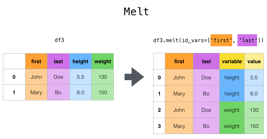
To perform a sanity check on our results, we will recreate the plot from notebook 1, but this time using categorical data types for the drought indicators. However, before we can plot this data, we need to reshape it into a “long” or “stacked” format. This format will allow us to use the groupby parameter of the hvplot extension for pandas. We will reshape the data using the pandas melt method, keeping the indexes and coordinates unchanged while stacking the indicator values. The variable column will identify the drought indicator.

df_long = df_wide_cat.melt(id_vars=["latitude", "longitude"], ignore_index=False)
df_long

		latitude	longitude	variable	value
time	location_id
2007-01-01	10234428	-26.855516	32.357162	spei	severe
	10235038	-26.849566	32.621094	spei	moderate
	10235648	-26.843615	32.885020	spei	NaN
	10236025	-26.839937	32.457973	spei	severe
	10236635	-26.833986	32.721905	spei	moderate
...	...	...	...	...	...
2021-12-01	12001792	-10.528863	40.454630	zscore	normal
	12001792	-10.528863	40.454630	zscore	normal
	12001792	-10.528863	40.454630	zscore	normal
	12001792	-10.528863	40.454630	zscore	normal
	12001792	-10.528863	40.454630	zscore	moderate

15135618 rows × 4 columns

Now we can plot the data, where we the datashader method by and any to deal with the new categorical data type when turning the data to a raster.

color_key = {
    "extreme": "#bb0c0c",
    "severe": "#c57b19",
    "moderate": "#b1bb29",
    "mild": "#1cd87a",
    "normal": "#ffffff",
}


legend = (
    df_long[~df_long.index.duplicated()]
    .dropna()
    .hvplot.points(
        x="longitude",
        y="latitude",
        c="value",
        groupby="time",
        color_key=color_key,
        crs=ccrs.PlateCarree(),
    )
)


map = df_long.hvplot.points(  # noqa: A001
    x="longitude",
    y="latitude",
    c="value",
    groupby=["variable", "time"],
    x_sampling=0.1,
    y_sampling=0.1,
    aggregator=ds.by("value", ds.any()),
    rasterize=True,
    crs=ccrs.PlateCarree(),
    tiles=True,
    frame_width=500,
    clabel="Drought anomaly",
    color_key=color_key,
    colorbar=False,
)
legend * map

12.6 Spatial Drought Extent Through Time

Now that we have classified drought intensity into categories, let’s calculate the spatial extent of droughts over time. This will enable us to compare how the two standardized drought indices relate to each other. Conveniently, we can use the pandas value_count method on the new categorical columns "spei" and "zscore", and also employ the normalize parameter to get relative frequencies. This provides an understanding of how many data points fall into each drought class relative to the total number of observations for a certain month.

col_spei = (
    df_wide_cat.groupby(level=0)["spei"].value_counts(normalize=True).unstack()  # noqa: PD010
)
col_zscore = (
    df_wide_cat.groupby(level=0)["zscore"].value_counts(normalize=True).unstack()  # noqa: PD010
)

We combine these relative frequencies results.

new_keys = pd.Index(["spei", "zscore"], name="indicator")
df_drought_extend = pd.concat(
    [col_spei, col_zscore],
    keys=new_keys,
)
df_drought_extend

		extreme	severe	moderate	mild	normal
indicator	time
spei	2007-01-01	0.000000	0.013475	0.037324	0.218705	0.730496
	2007-02-01	0.000000	0.000000	0.003304	0.266390	0.730305
	2007-03-01	0.000428	0.041281	0.176408	0.670018	0.111866
	2007-04-01	0.000000	0.015988	0.037592	0.381423	0.564997
	2007-05-01	0.065519	0.118397	0.153631	0.251963	0.410490
...	...	...	...	...	...	...
zscore	2021-08-01	0.006945	0.020372	0.061580	0.304501	0.606602
	2021-09-01	0.005529	0.018969	0.052673	0.342970	0.579859
	2021-10-01	0.003601	0.021911	0.073392	0.466220	0.434875
	2021-11-01	0.003094	0.013771	0.076638	0.583993	0.322505
	2021-12-01	0.073324	0.290879	0.318676	0.240002	0.077120

360 rows × 5 columns

As a final step we will plot the timeseries of the relative spatial extend of the upper three drought clases (“moderate”, “severe”, and “extreme”). We compare these results to recorded drought events that had a severe impact on food security and destabelized Mozambique.

mozambique_droughts = [
    {"time": "2008-01-01", "people_affected": 1.02},
    {"time": "2010-01-01", "people_affected": 0.46},
    {"time": "2016-01-01", "people_affected": 2.30},
    {"time": "2021-01-01", "people_affected": 1.56},
]

df_droughts = pd.DataFrame(mozambique_droughts).assign(y=1)
df_droughts["time"] = pd.to_datetime(df_droughts["time"], format="%Y-%M-%d")
df_droughts = df_droughts.set_index("time")
labels = df_droughts.hvplot.labels(
    x="time",
    y="y",
    text="{people_affected} mill. people",
    text_baseline="bottom_left",
    hover=False,
    angle=85,
    text_font_size="14px",
)
offset = hv.dim("y") - 0.1
points = df_droughts.hvplot.points(
    x="time", y="y", color="black", hover=False, transforms={"y": offset}
)
df_drought_extend.hvplot.area(
    x="time",
    y=drought_labels[::-1][2:],
    groupby="indicator",
    hover=False,
    frame_width=800,
    padding=((0.1, 0.1), (0, 0.9)),
) * labels * points

We observe significant differences between the two drought indicators. The SPEI drought information shows much higher variability compared to the Z-scores derived from H SAF ASCAT SSM data. We find that the spatial extent of the most severe drought classes, as indicated by the Z-scores, aligns well with recorded drought disasters.

The higher variability in SPEI might be due to the more variable precipitation input, while soil moisture has a “memory”, i.e. soil moisture represents water storage. Precipitation does not account for infiltration and overland flow. In SPEI the type of precipitation is not accounted for, and thus a very intense rainfall event, where a lot of rainfall falls in a short period, will not lead to a sustainable increase in soil water content, and plant available water, as most of the water will not infiltrate in the soil. Therefore, deviations from the norm are likely more subdued in soil moisture data than in SPEI but are more representative for plant available water and is intricately linked to agricultural practices that are crucial for food security in Mozambique.

12.7 A Comprehensive Comparison of Drought Indicators

To obtain a more comprehensive and accurate overview of H SAF ASCAT SSM in detecting agriculturally relevant drought events, we will compare it with an additional set of drought indicators. These indicators are monthly Z-scores calculated from different soil moisture estimates. The estimates are derived from in-situ observations, remotely sensed retrievals, or hydro-meteorological models

Dataset	Description	Key Features	Applications
ERA5	ERA5 is a reanalysis dataset produced by ECMWF that provides comprehensive global climate and weather data, including soil moisture.	- High spatial and temporal resolution - Derived from model simulations and observational inputs - Global coverage	- Climate research - Hydrological modeling - Agricultural applications - Drought monitoring - Water resource management
GLDAS	The Global Land Data Assimilation System (GLDAS) soil moisture dataset provides global estimates of soil moisture based on satellite observations, ground measurements, and model simulations.	- High-resolution and temporally consistent - Integrates various data sources - Developed by NASA and NOAA	- Hydrological modeling - Climate studies - Agricultural monitoring - Drought assessment - Water resource management - Environmental sustainability
ESA CCI	The ESA CCI (European Space Agency Climate Change Initiative) Soil Moisture project aims to provide long-term, consistent datasets of global soil moisture derived from satellite observations.	- Long-term and consistent datasets - Derived from satellite observations - Supports scientific research and policy-making	- Climate research - Hydrological modeling - Agricultural monitoring - Environmental sustainability - Food security studies

We have already prepared a dataset that includes all these drought indicators, along with the previously introduced SPEI and ASCAT data (previously labeled "zscore").

url = make_url("drought_indices-6_25_monthly.csv")
df_drought_indices = pd.read_csv(
    url,
    index_col=["time", "location_id"],
    parse_dates=["time"],
)
df_drought_indices

https://git.geo.tuwien.ac.at/api/v4/projects/1266/repository/files/drought_indices-6_25_monthly.csv/raw?ref=main&lfs=true

		longitude	latitude	ascat	era5	spei	gldas	cci
time	location_id
2007-01-01	10234428	32.357162	-26.855516	-0.227513	-1.177816	-1.563430	0.575884	NaN
	10235038	32.621094	-26.849566	-0.263700	-1.105393	-1.418305	0.510610	0.254604
	10235648	32.885020	-26.843615	-0.524645	-0.190537	NaN	NaN	NaN
	10236025	32.457973	-26.839937	0.048931	-1.105393	-1.502107	0.575884	NaN
	10236635	32.721905	-26.833986	0.100799	-1.025658	-1.427557	0.510610	0.254604
...	...	...	...	...	...	...	...	...
2021-12-01	11992443	40.540737	-10.611925	-1.532990	-0.732172	NaN	NaN	NaN
	11993430	40.377617	-10.603155	-1.312185	-0.732172	-1.170215	-0.656978	NaN
	11995027	40.478430	-10.588965	-1.512508	-0.732172	NaN	-0.656978	NaN
	11997611	40.416126	-10.566007	-1.333472	-0.732172	-1.141002	-0.656978	NaN
	12001792	40.454630	-10.528863	-1.303371	-0.732172	NaN	-0.656978	NaN

7567809 rows × 7 columns

To simplify the calculation of relative drought spatial extent, we will create two functions that loops over the different columns to perform the same analysis as before: 1) set the categorical drought type and 2) calculate relative drought extent.

def set_drought_cat_type(df: pd.DataFrame) -> pd.DataFrame:
    """Drought Severity Levels.

    Parameters
    ----------
    df: Pandas.DataFrame
        Data frame with continuos drought indicators.

    Returns
    -------
        Pandas.DataFrame: Data frame with discrete drought indicators

    """
    col_names = df.drop(columns=["longitude", "latitude"]).columns
    for name in col_names:
        min_border = df[name].min()
        max_border = df[name].max()
        thresholds = np.array(
            [
                min_border if min_border < -2 else -2.1,  # noqa: PLR2004
                -2,
                -1.5,
                -1,
                0,
                max_border if max_border > 0 else 0.1,
            ]
        )
        df[name] = pd.cut(df[name], thresholds, labels=drought_labels)
    return df


def calc_drought_areal_extend(df: pd.DataFrame) -> pd.DataFrame:
    """Areal Extent of Drought Severity Levels.

    Parameters
    ----------
    df: Pandas.DataFrame
        Data frame with discrete drought indicators.

    Returns
    -------
        Pandas.DataFrame: Data frame with normalize counts of drought levels

    """
    col_names = df.drop(columns=["longitude", "latitude"]).columns
    return pd.concat(
        [
            df.groupby(level=0)[col].value_counts(normalize=True).unstack()  # noqa: PD010
            for col in col_names
        ],
        keys=pd.Index(col_names, name="indicator"),
    )


df_drought_indices_cat = set_drought_cat_type(df_drought_indices.copy())
df_drought_extend = calc_drought_areal_extend(df_drought_indices_cat)
df_drought_extend.hvplot.area(
    x="time",
    y=drought_labels[::-1][2:],
    groupby="indicator",
    hover=False,
    frame_width=800,
    padding=((0.1, 0.1), (0, 0.9)),
) * labels * points

The additional drought indicators share the characteristic of directly measuring or estimating the soil’s water content by modeling soil geophysical conditions. This comparison validates the earlier observation that the SPEI-inferred drought extent exhibits greater variability compared to indicators based on soil moisture. However, with the exception of the H SAF ASCAT SSM-derived Z scores, all indicators show significant discrepancies in their estimates of drought extent for the five major drought events.

12.8 Close-up of the 2015–2016 (El Niño) Drought Event

Let’s now zoom in on one of the most significant drought disasters of recent history in Mozambique. The 2015-2016 drought event which has been related to El Niño significantly impacted agriculture, food security, and water resources. This drought was characterized by reduced rainfall and elevated temperatures, exacerbating conditions for farming and livestock. Estimated numbers for people affected by this events are ~2.3 million.

We filter this event from the loaded dataset and plot as before with hvplot.

df_long_2016 = df_drought_indices_cat.loc["2016-01-01"].melt(
    id_vars=["latitude", "longitude"], ignore_index=False
)

legend_2016 = (
    df_long_2016[~df_long_2016.index.duplicated()]
    .dropna()
    .hvplot.points(
        x="longitude",
        y="latitude",
        c="value",
        color_key=color_key,
        crs=ccrs.PlateCarree(),
    )
)

map_2016 = df_long_2016.hvplot.points(
    x="longitude",
    y="latitude",
    c="value",
    groupby=["variable"],
    x_sampling=0.1,
    y_sampling=0.1,
    aggregator=ds.by("value", ds.any()),
    rasterize=True,
    crs=ccrs.PlateCarree(),
    tiles=True,
    frame_width=500,
    clabel="Drought anomaly",
    color_key=color_key,
    colorbar=False,
)
legend_2016 * map_2016

A visual inspection of the map displaying various drought indicators reveals broad similarities, with most indicators highlighting drought conditions in the southern provinces of Maputo and Gaza, as well as in Sofala, Tete, and Zambezia. However, the spatial patterns also exhibit significant differences in their finer details. These discrepancies are likely influenced by the inherently coarser resolutions of ERA5 (9 km), ESA CCI, and GLDAS (~25 km).

S. M. Vicente-Serrano, S. Begueria, and J. I.López-Moreno,A Multiscalar Drought Index Sensitive to Global Warming: The Standardized Precipitation Evapotranspiration Index, Journal of Climate, vol. 23, no. 7, pp. 1696-1718, Apr. 2010, doi: 10.1175/2009JCLI2909.1.↩︎
T. B. McKee, N. J. Doesken, and J. Kleist, The Relationship Of Drought Frequency and Duration to the Timescale. Eighth Conference on Applied Climatology, 17-22 January 1993, Anaheim, California↩︎