13 Leads and lags in Drought Dynamics – Earth Observation Datascience

Meteorological, Agricultural, and Hydrological Droughts

13.1 Overview

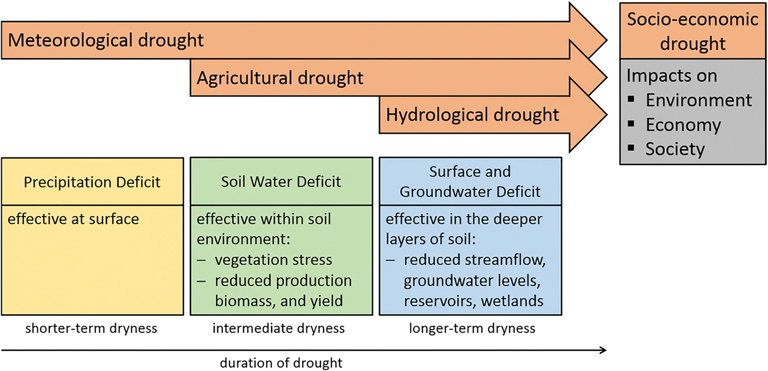
In this notebook we will examine the propagation of precipitation deficits, soil water deficits, and finally their lagged effect on plants. This cascading effect of drought development, or so-called convergence of evidence, is important to study in areas where rain-fed agricultural practices are of importance, such as Mozambique.

Classically drought have been categorized in four classes:

Meteorological drought is described as the lack of precipitation and/or increased atmospheric demand (evapotranspiration)
Agricultural drought is also a physical phenomenon where soils become replete of moisture
Hydrological drought follows when ongoing drought can then cause deficits in ground and surface reservoirs
Socioeconomic drought impacts society through crop loss, food insecurity, shortages of fresh-water resources

The first three phenomena often follow in a cascading sequence, whereas all of them can have a direct impact on society.

import hvplot.pandas  # noqa
import pandas as pd
import statsmodels.formula.api as smf
import statsmodels.tsa.stattools as smt
from envrs.corr_plots import plot_step_corr, plot_predicted_values
from envrs.download_path import make_url

Resolve path ffmpeg: /home/runner/work/eo-datascience/eo-datascience/.conda_envs/environmental-remote-sensing/bin/ffmpeg

13.2 Monitoring Drought Dynamics

To track drought development in this exercise we will work with precipitation, soil moisture and vegetation data. The following dataset combines the HSAF ASCAT 6.25 surface soil moisture with data for precipitation from CHIRPS, and data for vegetation, the NDVI (see table).

Feature	NDVI (Normalized Difference Vegetation Index)	CHIRPS (Climate Hazards Group InfraRed Precipitation with Station data)
Description	A widely used index to measure the health and vigor of vegetation (“greenness” of the biomes).	A high-resolution precipitation dataset that combines satellite and station data.
Data Source	Remote sensing, typically from satellite imagery.	Satellite infrared data combined with rain gauge station data.
Calculation	(NIR - RED) / (NIR + RED), where NIR is Near-Infrared and RED is Red light reflectance.	Combines data from multiple sources to provide daily precipitation estimates.
Applications	- Agriculture: Monitoring crop health and growth. - Ecology: Assessing vegetation cover and changes. - Climate: Studying vegetation response to climate change.	- Drought monitoring and early warning. - Hydrological modeling. - Agricultural planning and risk management.
Advantages	- Simple and quick to calculate. - Provides a standardized measure of vegetation health. - Useful for temporal and spatial comparisons.	- High spatial and temporal resolution. - Integrates multiple data sources for better accuracy. - Useful for regions with sparse rain gauge networks.
Limitations	- Sensitive to atmospheric conditions and soil background. - May require calibration for different vegetation types. - Does not distinguish between different types of vegetation.	- Dependent on the quality and availability of input data. - May have errors in areas with complex terrain or dense vegetation. - Requires validation with ground truth data.
Use Cases	- Detecting areas of stressed or unhealthy vegetation. - Monitoring deforestation and land use changes. - Assessing the impact of droughts and floods on vegetation.	- Providing real-time precipitation data for disaster response. - Supporting water resource management and irrigation planning. - Enhancing climate models and weather forecasting.

In summary, NDVI indicates plant health based on the assumption that plants lose their greenness when they wilt due to water deprivation. However, this signal is highly dependent on vegetation types, soil background, and atmospheric conditions. CHIRPS measures precipitation and is affected by the quality of the input data, which can be problematic if there is a scarcity or poor quality of meteorological stations in a region.

Let’s load the data as prepared for the notebook.

url = make_url("drought_indices-6_25_dekadal.csv")
df_dekadel = (
    pd.read_csv(
        url,
        index_col="time",
        parse_dates=True,
    )
    .dropna()
    .sort_index()
)

df_dekadel.head()

https://git.geo.tuwien.ac.at/api/v4/projects/1266/repository/files/drought_indices-6_25_dekadal.csv/raw?ref=main&lfs=true

	longitude	latitude	surface_soil_moisture	ndvi	precip	name
time
2012-01-01	34.770840	-18.889309	0.30570	0.564	0.046854	Muanza
2012-01-01	32.540100	-23.426407	0.29010	0.432	0.002876	Mabalane
2012-01-01	34.113262	-22.077436	0.31970	0.576	0.020926	Mabote
2012-01-01	34.119698	-19.975350	0.31385	0.576	0.024297	Buzi
2012-01-01	33.030777	-24.612324	0.19315	0.320	0.000000	Chokwé

We have five time series datasets spanning from 2011 to 2020 for the selected locations in the DrySat project, available for in-depth analysis (refer to notebooks 1 and 2). The NDVI data is sourced from the Copernicus Land Monitoring Service, and the CHIRPS data is obtained from ClimateSERV. NDVI values range from 0 to 1 and are often classified as follows:

0 to 0.1: Bare soil, rock, or sand.
0.1 to 0.2: Low vegetation or senescent (dying) vegetation.
0.2 to 0.5: Sparse vegetation, such as shrubs and grasslands.
0.5 to 0.7: Moderate to high vegetation, such as crops and forests.
0.7 to 1: High density of green leaves, indicative of very healthy vegetation.

For this analysis, the ASCAT H SAF surface soil moisture (SSM) data, originally at a 6.25 km resolution and expressed as a percentage of saturation, is converted to a unit scale ranging from 0 to 1. Additionally, the CHIRPS precipitation data, measured in millimeters, is min-max scaled for each location’s time series individually to also range between 0 and 1.

Both NDVI and CHIRPS datasets are natively 10-daily products (or ‘dekadal’), while the SSM data is resampled to match this dekadal frequency.

Let’s have a look at the data for each site individually with hvplot use the dropdown menu “name” to select the preferred site.

df_dekadel.hvplot.line(
    x="time",
    y=["precip", "surface_soil_moisture", "ndvi"],
    subcoordinate_y=True,
    groupby=["name"],
    frame_width=800,
)

By examining the three variables—CHIRPS precipitation (precip), H SAF surface soil moisture (surface_soil_moisture), and NDVI (ndvi)—we observe a strong temporal correlation among them. This correlation is logical, as we expect rain to wet the soil, which in turn nourishes plant life, and vice versa. The most significant changes in these variables appear to be linked to transitions between dry and wet seasons.

13.3 Exploration with Linear Regression

Let’s delve deeper into the relationships among these three variables. Linear regression, specifically Ordinary Least Squares (OLS) regression, is a powerful tool for explanatory data analysis. OLS is a good starting point for your analysis as it is easy to interpret; the coefficients directly relate changes in the response variable to one-unit changes in the predictor variables, with the sign and magnitude reflecting the model’s effects. In an OLS regression, these effects refer to the impact of the independent variables on the dependent variable.

Although the assumptions underlying OLS regression (such as linearity, independence of observations, and normality of residuals) are likely to be violated, especially in time series analysis where observations closely spaced in time are likely to be dependent on each other (autocorrelation), we can still use OLS for an ad hoc analysis of the previously observed physical relationships. Specifically, we aim to test the following relationships:

More rain leads to healthier vegetation.
Wetter soils lead to healthier vegetation.

These relationships are intuitively important causal factors. To determine which best explains the dependent variable (NDVI), we will perform OLS regression using the statsmodels package. Note that other Python packages, like scipy.stats, are also available.

We’ll utilize statsmodels’ formula interface, which allows specifying models with formula strings and directly using pandas.DataFrames. This interface employs a tilde (~) to separate the dependent variable from the independent variables. Interactions between variables can be specified using the * or : operators, enabling easy expansion to multiple regression. It also simplifies variable transformations and polynomial terms.

To translate the OLS equation:

\[\text{NDVI} = \alpha + \beta \text{CHIRPS} + \epsilon \]

into an statsmodels formula, you use:

df_buzi = df_dekadel[df_dekadel.name == "Buzi"]
mod_precip = smf.ols(formula="ndvi ~ precip", data=df_buzi)

In this context, ndvi is the dependent variable, precip is the independent variable, and df_buzi is the data frame containing your data. We will focus on the Buzi region for the OLS regression and subsequent analysis.

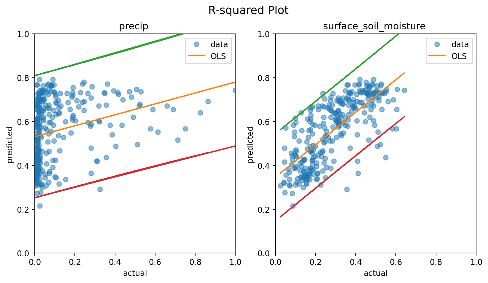
To fit the model, simply call the fit method on the generated object. We will then print the parameters and their estimated coefficients as well as the variation in NDVI explained by the \(R^2\) value.

res_precip = mod_precip.fit()

print("Parameters: \n", res_precip.params, sep="")
print("R2: ", res_precip.rsquared)

Parameters: 
Intercept    0.531179
precip       0.249106
dtype: float64
R2:  0.08314849453004114

We can see that the model fit with CHIRPS precipitation as independent variable is limited. Now let’s do the same for the second predefined relationship, where we translate (\(\text{NDVI} = \alpha + \beta \text{SSM} + \epsilon\)) into an statsmodels formula and asses it’s fit, like so:

mod_ssm = smf.ols(formula="ndvi ~ surface_soil_moisture", data=df_buzi)
res_ssm = mod_ssm.fit()

print("Parameters: \n", res_ssm.params, sep="")
print("R2: ", res_ssm.rsquared)

Parameters: 
Intercept                0.346452
surface_soil_moisture    0.740606
dtype: float64
R2:  0.5374351087887564

This approach provides better results, explaining nearly 50% of the variance in NDVI with H SAF ASCAT SSM. Additionally, we can visualize these results using an \(R^2\) plot to perform a more detailed diagnostic analysis of the model’s performance. We have predefined and loaded this function at the top of the notebook for clarity.

results = {"precip": res_precip, "surface_soil_moisture": res_ssm}
plot_predicted_values(
    df_buzi,
    results,
    figsize=(10, 5),
)

13.4 Leads and Lags of Water Availability and Vegetation

At the beginning of the notebook, we highlighted that droughts are cascading events where a lack of rain leads to reduced soil moisture, which in turn affects plant health. To study the dynamics of these cascading droughts, we should first examine the effects of precipitation and soil moisture on vegetation under normal conditions. We need to consider both the lead and lag of the respective causes and effects in this system. Precipitation leads, soil moisture replenishment lags, and vegetation responds with a delay to rainfall events.

Though the cyclical nature of NDVI, H SAF ASCAT SSM, and CHIRPS precipitation is evident, these cycles correspond to the dry and wet seasons experienced in Mozambique. To quantify the actual periodicity of these seasons, autocorrelation is a useful tool. Autocorrelation in time series refers to the correlation of a time series with a delayed copy of itself, measuring the extent to which a time series value is linearly related to its past and future values. The following animation visually demonstrates how a copy of the time series is shifted alongside itself, illustrating the corresponding correlation, known as autocorrelation. This can be expressed as:

\[r_k = \frac{\sum_{t=1}^{N-k}{(x_t-\bar{x} )(x_{t+k} -\bar{x})}}{\sum_{t=1}^N{(x_t-\bar{x}})}\]

plot_step_corr(df_buzi, "ndvi", length=72)

As expected, it takes 18 lags (or 18 dekads, equivalent to approximately half a year) for the signal to become almost entirely anti-correlated. It then takes 36 lags (or 36 dekads, equivalent to approximately 1 year) for the cycle to complete and the signal to become almost perfectly correlated again. You can perform you own autocorrelation test with statsmodels, like so:

smt.acf(df_buzi.ndvi, nlags=4)

array([1.        , 0.94896775, 0.88434477, 0.79925742, 0.69430392])

Similarly, we can compare the lagged time series of CHIRPS precipitation with NDVI and the lagged time series of H SAF ASCAT SSM with NDVI. This type of analysis is known as lagged cross-correlation analysis. The following two animations illustrate the cross-correlations of H SAF ASCAT SSM with NDVI and CHIRPS precipitation with NDVI respectively.

plot_step_corr(df_buzi, "ndvi", "precip", length=72)

plot_step_corr(df_buzi, "ndvi", "surface_soil_moisture", length=72)

We observe that these wet-dry cycles do not perfectly align among the two variables in our analysis. In both cases, the correlation initially increases with 3 to 6 lags in the time series for CHIRPS precipitation and H SAF SSM, respectively.

NDVI lags CHIRPS precipitation by 6 dekads (or approximately 2 months).
NDVI lags H SAF SSM by 3 dekads (or approximately 1 month).

You can again perform you own lagged cross-correlation test with statsmodels, like so:

smt.ccf(df_buzi.ndvi, df_buzi.surface_soil_moisture, nlags=4)  # for example

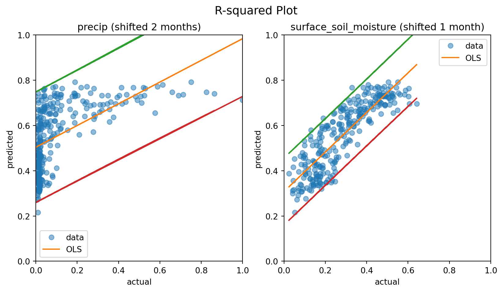
array([0.73309966, 0.82333965, 0.86011595, 0.87138539])

13.5 Lagged Variable Regression

Now that we’ve determined the appropriate lag, we can revisit the OLS regression. By using pandas’ shift function, we adjust precip and surface_soil_moisture accordingly and then apply the statsmodels OLS regression to the lagged dataset.

df_buzi_shift = df_buzi.assign(
    surface_soil_moisture=df_buzi.loc[:, "surface_soil_moisture"].shift(3),
    precip=df_buzi.loc[:, "precip"].shift(6),
).dropna()

df_buzi_shift

	longitude	latitude	surface_soil_moisture	ndvi	precip	name
time
2012-03-01	34.119698	-19.97535	0.26675	0.608	0.024297	Buzi
2012-03-11	34.119698	-19.97535	0.27485	0.636	0.375177	Buzi
2012-03-21	34.119698	-19.97535	0.13000	0.580	0.154025	Buzi
2012-04-01	34.119698	-19.97535	0.36055	0.688	0.053977	Buzi
2012-04-11	34.119698	-19.97535	0.29830	0.676	0.244914	Buzi
...	...	...	...	...	...	...
2019-11-11	34.119698	-19.97535	0.13205	0.336	0.022271	Buzi
2019-11-21	34.119698	-19.97535	0.15360	0.528	0.020403	Buzi
2019-12-01	34.119698	-19.97535	0.17110	0.544	0.074502	Buzi
2019-12-11	34.119698	-19.97535	0.20390	0.600	0.009415	Buzi
2019-12-21	34.119698	-19.97535	0.30400	0.632	0.035159	Buzi

282 rows × 6 columns

Thee lagged values of precipitation to account for the delayed impact of rainfall on vegetation health would look something like this:

\[ \text{NDVI}_t = \alpha + \beta \text{CHIRPS}_{t-6} + \epsilon_t \]

In this equation, \(\text{NDVI}_t\) is the dependent variable at time \(t\) and \(\text{CHIRPS}_{t-6}\) is the 6 dekadal lagged independent variables with \(\beta\) as the coefficient. This approach can provide insights into how past events influence current outcomes, making it a valuable tool for time series analysis. We implement this as follows:

mod_precip_shift = smf.ols(formula="ndvi ~ precip", data=df_buzi_shift)
res_precip_shift = mod_precip_shift.fit()

print("Parameters: \n", res_precip_shift.params, sep="")
print("R2: ", res_precip_shift.rsquared)

Parameters: 
Intercept    0.503815
precip       0.479969
dtype: float64
R2:  0.3076670920100214

We observe that including lagged rainfall data improves the model fits compared to a model without this information. Next, we will apply the same approach to H SAF SSM, now using a time lag of 3 dekads:

mod_ssm_shift = smf.ols(formula="ndvi ~ surface_soil_moisture", data=df_buzi_shift)
res_ssm_shift = mod_ssm_shift.fit()

print("Parameters: \n", res_ssm_shift.params, sep="")
print("R2: ", res_ssm_shift.rsquared)

Parameters: 
Intercept                0.307934
surface_soil_moisture    0.874578
dtype: float64
R2:  0.74824179183522

Here again the model fit improves over the model without lagged variables. We can perform a sanity check by plotting again the \(R^2\) plots.

results_shift = {"precip": res_precip_shift, "surface_soil_moisture": res_ssm_shift}
plot_predicted_values(
    df_buzi_shift,
    results_shift,
    figsize=(10, 5),
    suffix=["(shifted 2 months)", "(shifted 1 month)"],
)

These \(R^2\) plots indicate that the relationships are better captured with lagged variables compared to unlagged ones. However, the precipitation data does not fully conform to the underlying principles of linear regression with OLS. It is quite obvious from this plot that rainfall data contains a lot of zeros. This should be addressed before one can make inferences from the model.

13.6 Enhancing the Robustness of Lagged Variable OLS Analysis

To advance the lagged variable analysis with Ordinary Least Squares (OLS), we need to consider several methodological enhancements. Here are strategies to take this forward:

BLUE Estimators: Ensure your models conform to the properties of BLUE estimators (Bias, Linearity, Uncorrelated errors, and Efficiency). This will provide the most reliable and unbiased estimates for your regression coefficients.
Autocorrelation: Autocorrelation can significantly affect the reliability of your model. We’ve already identified strong autocorrelation in the temporal domain using autocorrelation tests. Consider looking into Generalized Least Squares models, which can account for dependency structures in their residuals.
Multiple Independent Variables: Incorporate multiple independent variables, including both lagged and unlagged versions. For example, include precipitation, soil moisture, and other relevant factors with appropriate lag structures to capture their delayed effects.
Non-normal Residuals: If your residuals are not normally distributed, it can impact the validity of your hypothesis tests. Techniques such as transforming the dependent variable (e.g., using log or Box-Cox transformations), or using robust regression methods can help address this.
Non-linear Behavior: If you detect non-linear relationships, consider using polynomial regression or non-linear regression models. Interaction terms between your independent variables can also capture non-linear effects within an OLS framework.
Model Diagnostics: Regularly perform diagnostic checks on your models. Examine plots of residuals versus fitted values, histograms of residuals, and autocorrelation plots to ensure model assumptions are met and identify areas for improvement.

By adopting these strategies, you will significantly enhance the robustness of your lagged variable OLS analysis, ensuring it is both methodologically sound and practically useful for understanding and predicting complex dynamic systems. Ultimately, this will help us better comprehend the normal wet/dry dynamics of the system, allowing us to predict the effects of current drought conditions on crops and subsequently help forecast yield.

L. Crocetti et al., Earth Observation for agricultural drought monitoring in the Pannonian Basin (southeastern Europe): current state and future directions, Reg Environ Change, vol. 20, no. 4, p. 123, Dec. 2020, doi: 10.1007/s10113-020-01710-w.↩︎