ERROR 1: PROJ: proj_create_from_database: Open of /home/runner/work/eo-datascience/eo-datascience/.conda_envs/environmental-remote-sensing/share/proj failed
14.3 H SAF
H SAF, the Satellite Application Facility on Support to Operational Hydrology and Water Management, is part of EUMETSAT, the ‘European Organisation for the Exploitation of Meteorological Satellites’ headquartered in Darmstadt, Germany. EUMETSAT consists of 30 European Member states and operates both geostationary satellites (Meteosat) and polar-orbiting satellites (Metop), the latter of which carry the ASCAT sensors used for soil moisture retrieval. These missions are crucial for weather forecasting and significantly contribute to environmental and climate change monitoring. H SAF aims to disseminate satellite-derived products useful for operational hydrology, including precipitation, snow cover, and soil moisture. They ensure that these products are accurate through rigorous validation and are delivered to users in a timely manner. All these products are freely available.
14.4 Registration
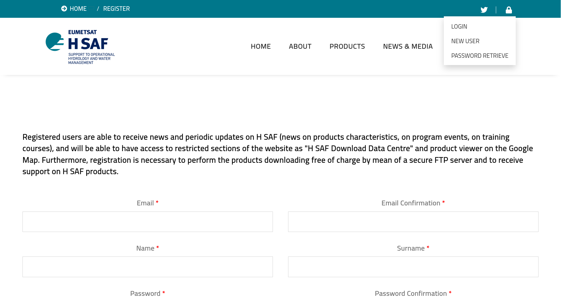
H SAF has an FTP server for users to download near real time data products. Before you can start downloading data products, one need to register to become an H SAF user. This is relatively easy when following these steps:
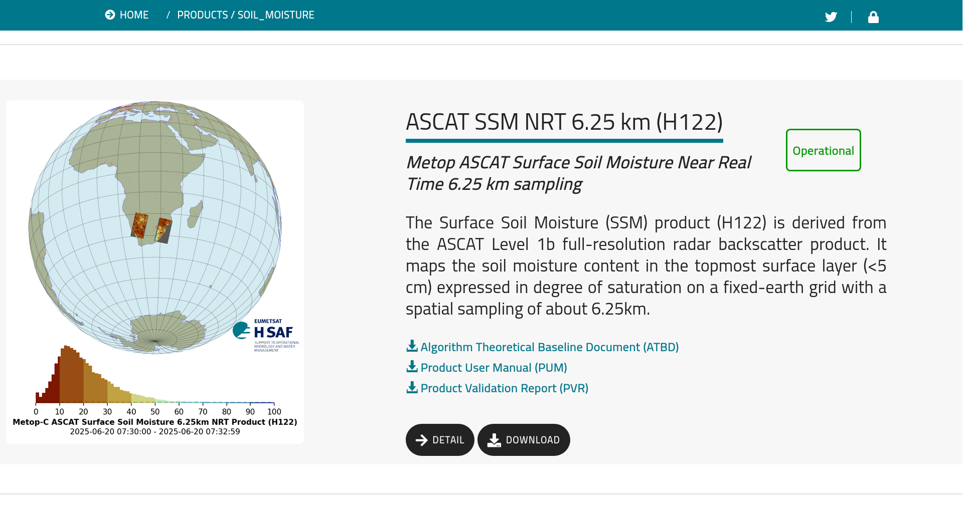
You can then click on “Download”. This will provide you with the URL of the FTP server for downloading.
14.5 Downloading
Now that we have the address for finding the soil moisture data products in the form of an URL, we need to think about a method to download the data. In other words we need a client, which requests the resources from the H SAF FTP servers. One way to download the data would be to use a client with a graphical user interface, like FileZilla.
Of course, we will look into a “Pythonic” way to download the data. For this we use the ascat package developed by the TU Wien. You can pip install this package from the Python Package Index (PyPi), like so:
pip install ascat
The ascat package has a download interface hsaf_download. The interface needs the following information; a local path for saving the downloaded data, a remote path to locate the H SAF data products on the FTP server, and a start and end datetime for the query. Here we show how to download the H SAF SSM 6.25 km product for the last 30 days from the time of running this notebook.
You also need to provide your credentials to authenticate with the FTP server, which you obtained when registering as an user (see above). It is always a good practice to “not” store your credentials, tokens, and other secrets in scripts or notebooks. Hence, we will use a dotenv (.env). Dotenv is a tool that helps load environment variables from an .env-file into your application’s environment, allowing you to manage configuration settings separately from your code.
Before you can use dotenv, you will have to create the .env-file manually or with the command line, like so
touch .env
Open the file and write your email at the location indicated with <your_email_here> and your password here: <your_password_here>.
2025-10-05 15:31:57,644 INFO: FTP connection successfully established
2025-10-05 15:32:40,671 INFO: FTP disconnected
CPU times: user 354 ms, sys: 185 ms, total: 539 ms
Wall time: 44.2 s
14.6 Swath vs. Cell Format Soil Moisture Data
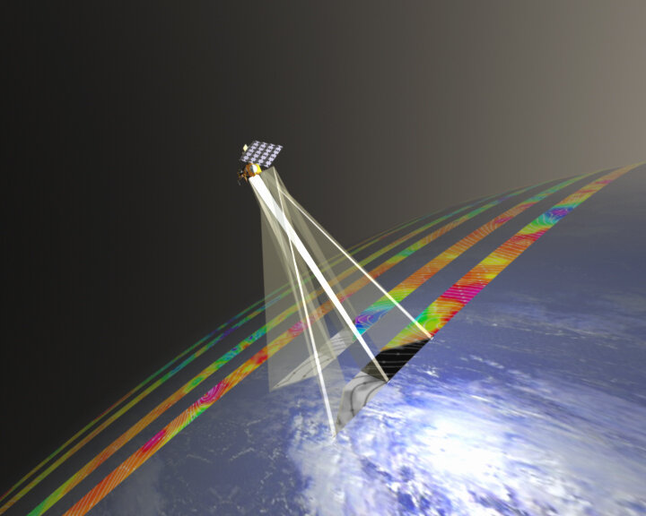
The data provided by the near real time service is provided in “swath” format as opposed to the “cell” format with which we worked before. A swath is the area on the Earth’s surface that is observed or imaged by a satellite or an airborne sensor during a single pass. This is often visualized as a strip or a corridor of data collected as the satellite or aircraft moves along its path (see figure below).
Distinctive double strips when ASCAT scans the Earth’s surface (Source: ESA)
Each format has its unique characteristics and implications for Earth observation research:
Precision agriculture, local hydrological studies, detailed environmental monitoring
In summary, the choice between swath and cell formats depends on the specific requirements of the Earth observation research. Swath data is advantageous for broad, frequent coverage, while cell data offers detailed, localized information.
Let’s have a look at the downloaded swath data. For this we can use again the ascat package and the SwathGridFiles class where point to the downloaded data and provide the product id "H130". We can then read the data, which return the ASCAT 6.25 km data in swath format as a Pandas.DataFrame.
The DataFrame now includes additional columns when compared with earlier notebooks. These columns indicate that the data is accompanied by quality flags to ensure the reliability and accuracy of soil moisture estimates for specific studies and areas of interest. Users have to use these flags to filter out unreliable data to maintain an accurate overview of the conditions.
For the data used in these notebooks, specific flags and threshold values were applied: “topographic_complexity” and “wetland_fraction” were set below 20%. This is because the backscattering of microwaves from topographically varied terrain, such as hills, valleys, and slopes, creates surface roughness that can scatter the microwave signal in multiple directions. This scattering leads to a more complex and less predictable backscatter signal. Additionally, wetland backscattering signals can be dominated by water, resulting in biased soil moisture retrievals. This bias can be further compounded by microwaves bouncing off water surfaces into reed belts and other vegetation along the shores of water bodies. To ensure sufficient variation in the backscatter signal, the sensitivity flag is set to more than 1 dB (decibel), allowing the retrieval algorithms to separate soil moisture contributions from noise. It is expected that in Mozambique, vegetation attenuation of microwaves can create unfavorable conditions for soil moisture retrievals due to this mechanism.
There are many more processing and quality flags. Check the ASCAT Soil Moisture User Manual for the other flags and determine if they are important for your requirements.
By applying these quality flags and understanding their implications, users can better interpret the soil moisture data and ensure that their analyses are based on reliable and accurate information. This approach helps mitigate the potential biases introduced by topographic complexity and wetland influences, ultimately leading to more robust and informative soil moisture retrievals.
14.8 Selecting a Region of Interest
We will plot the obtained soil moisture data without applying any filters. We use hvplot, as we typically do. It is evident that the “swath” format data provides global coverage. However, this format makes it more challenging to directly download data specific to your area of interest, such as Mozambique. To target a specific region before downloading the data, one needs to understand the intersection of the swath geometry with the area of interest at any given time. This is beyond the scope of this course. At present you can download the whole swaths and then extract the region of interest.
Note, that one can stack swath format data to obtain cell format data. This functionality is available in the ascat package, but this is beyond the scope of this notebook.