In this notebook we will examine how one can obtain historic soil moisture data. We will do this by looking into the Copernicus WEkEO portal.
15.2 Imports
from pathlib import Pathimport cartopy.crs as ccrsimport hvplot.pandas # noqaimport numpy as npimport pandas as pdimport xarray as xrfrom dotenv import dotenv_valuesfrom hda import Client, Configurationfrom numpy.lib.recfunctions import unstructured_to_structuredfrom pyswi.swi_ts import calc_swi_tsfrom envrs.download_path import make_urlfrom envrs.ssm_cmap import SSM_CMAP
ERROR 1: PROJ: proj_create_from_database: Open of /home/runner/work/eo-datascience/eo-datascience/.conda_envs/environmental-remote-sensing/share/proj failed
15.3 Copernicus WEkEO
The name WEkEO (pronounced [wikio]) refer to the four key organisations – EUMETSAT, ECMWF, Copernicus Programme, and Mercator Ocean International, which link to the broader user community (“WE”), with the purpose of knowledge advancement and sharing (“k”), focussing Earth and Environmental Observation (“EO”).
The platform is a web-based service that helps people easily access and use Earth observation data. Its main goal is to make it simple for researchers, companies, and decision-makers to get the data they need and analyze it without needing advanced tools or a lot of technical knowledge.
15.4 Registration
Similarly to H SAF FTP server, we need to register as an user to make full use of WEkEO, although some features are available without an account. We can follow these steps:
Click on top right “Login” button, whereafter we select “Create an account” and fill out the form.
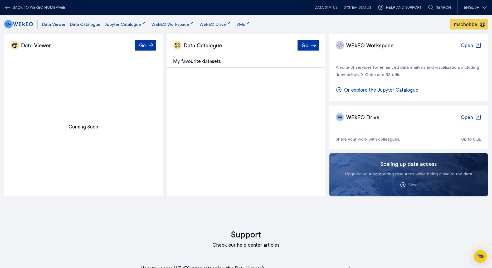
Now we can login and, for example, look at the available data by clicking on “Go” in the “Data Catalogue” field in the middle of the screen.
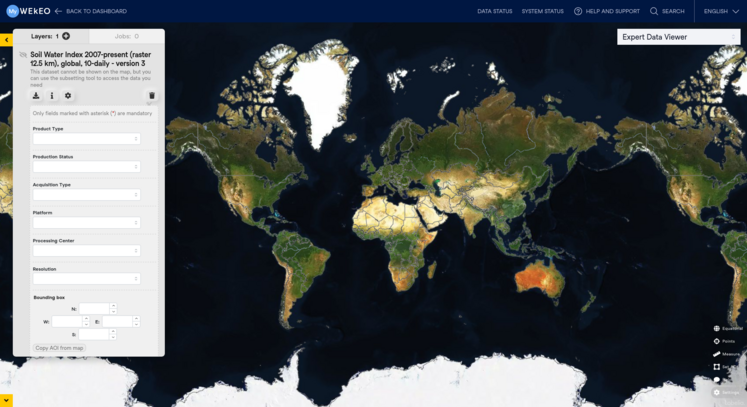
This shows us a data viewer where we can select from many different data products.
We will use the latter step to find the datasets we need and create query strings that we will use in a Python environment.
15.5 Harmonized Data Access
The Copernicus WEkEO platform offers a straightforward way to access data through its Application Programming Interface (API). APIs enable different programming languages to communicate and exchange information, effectively serving as a bridge for programs to utilize and extend each other’s functionalities. In the case of WEkEO, the API is called the Harmonized Data Access (HDA) API, which provides uniform access to the entire WEkEO catalogue, including subsetting and downloading capabilities. We will use the Python HDA client to interact with this API.
Install with either pip:
pip install hda
or conda:
conda install -c conda-forge hda
Now, we need to authenticate using the Configuration object and provide your account’s username and password. As in the previous notebook, we will use a dotenv environment for this purpose. To utilize dotenv, you need to add your username to the USER_WEKEO variable and your password to the PASS_WEKEO variable in the .env file.
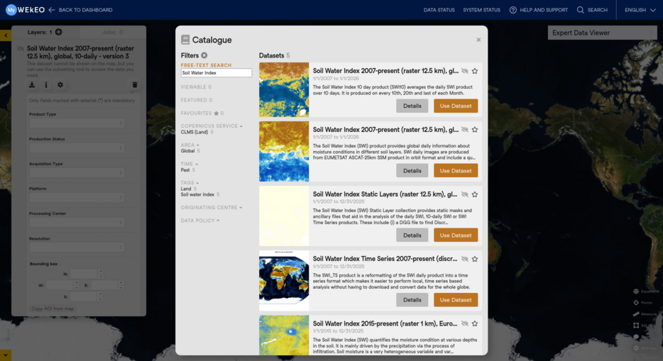
To find the SWI 12.5 km dataset in time series format, we have to return to the data viewer in the browser. Click in the “Layers” field on the + sign, and search for “Soil Water Index” in the “Free Text Search”.
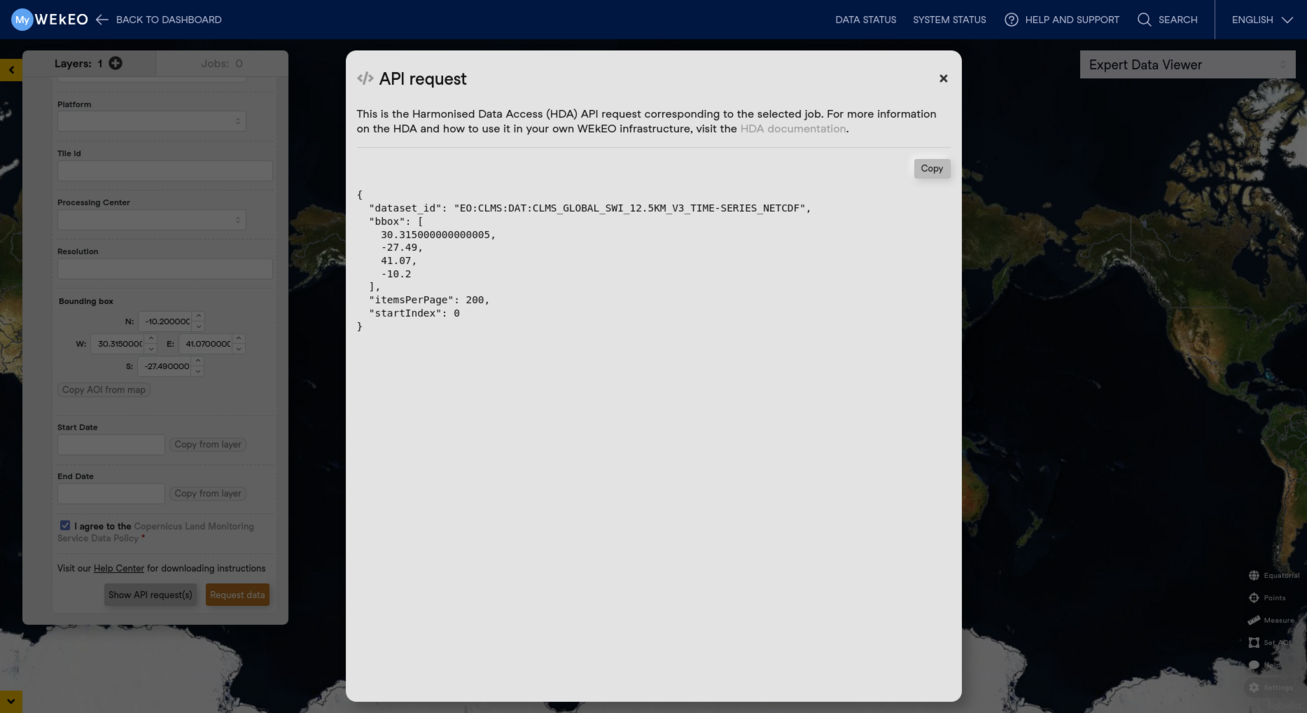
Then select the fourth dataset from the top; “Soil Water Index Time Series 2007-present (discrete global grid), global, daily - version 3”. Click on the download button in the layers field, which unfolds a form which allows subsetting of the data. We can enter here a bounding box (bbox) for Mozambique. Scroll further down and click on “Show API request(s)”.
We will copy this query to our Python environment and use the hda_client to search for the files.
If you are content with the results then you can start the downloading process. Here we again create a directory to contain the downloaded files. The downloaded file with be in NetCDF format. NetCDF is a data formats that is tailored to multi-dimensional array-oriented scientific data with many options to label the data.
The downloaded data is projected on the same Fibonacci grid as the H SAF ASCAT 6.25 km surface soil moisture (see notebook 1). But the NetCDF data format requires another solution to read the data. Hence we will use another package to read the data. We use xarray, which is optimised to work with multi-dimensional arrays. We will introduce this package into more detail later on. We will call the method to_dataframe() to turn the xarray.Dataset into a pandas.DataFrame.
We have not yet talked about what the data exactly represents. The Soil Water Index is derived from surface soil moisture. The current dataset is derived from H SAF ASCAT 12.5 km and represents modelled approximation of soil water content at deeper layers of the soil. In the above plot we selected moisture content at a 10 cm depth interval. Remember that ASCAT can only probe the surface of soils.
The Soil Water Index provides a measure of how wet or dry the soil is over a specific area, ranging between 0 and 1. It is often derived using a combination of satellite data and modeling techniques. One commonly used approach to derive the SWI is through the TU Wien model1
The equation to derive the SWI typically involves a convolution of surface soil moisture observations with an exponential filter. This process helps in estimating the root-zone soil moisture, which is more relevant for agricultural and hydrological applications. The general form of the equation can be described as follows:
\[
\begin{aligned}
\text{SWI} &\quad \text{: Soil Water Index} \\
\text{SSM}_i &\quad \text{: surface soil moisture at time step} i \\
w_i &\quad \text{: the weight assigned to the surface soil moisture at time step} i \\
n &\quad \text{: number of time steps considered in the convolution}
\end{aligned}
\]
The weights \(w_i\) are often determined using an exponential decay function, which gives more importance to recent observations. The exponential decay function can be expressed as:
\[ w_i = e^{-\frac{t_i}{T}} \]
Where: \[
\begin{aligned}
t_i &\quad \text{: the time difference between the current time step and the time step} i \\
T &\quad \text{: a characteristic time scale that determines the rate of decay of the weights}
\end{aligned}
\]
This approach allows the SWI to reflect the cumulative effect of surface soil moisture over a period, providing a more stable and representative measure of the soil moisture conditions in the root zone.
One will observe that the SWI at depth is often less variable (more stable) than contemporaneous surface soil moisture with only delayed and dampened responses to external forcing (e.g. precipitation). We can visualize this by applying the SWI algorithm to one of the five timeseries introduced in notebook 1.
Let’s select only the year 2024 from the H SAF ASCAT 6.25 km surface soil moisture for Buzi:
Now we can use the TU Wien developed package pyswi to calculate time series SWI. First we have to prepare the numpy arrays for the SSM and Julian time stamps2, like so:
After which, we convert the numpy arrays back to a pandas DataFrame and merge it with the original SSM data. This requires the Julian time steps to be converted back to a normal pandas datetime type.
W. Wagner, Lemoine, G., Rott, H., 1999, A Method for Estimating Soil Moisture from ERS Scatterometer and Soil Data, Remote Sensing of Environment, Volume 70-2, pp. 191-207, doi: S0034-4257(99)00036-X↩︎
Julian time stamps, also known as Julian dates, are continuous counts of days and fractions of days since a specific starting point, commonly used in astronomy and scientific applications to measure time intervals precisely.↩︎