from enum import Enum
from pathlib import Path
from typing import Any
import geopandas as gpd
import hvplot.pandas
import hvplot.xarray # noqa
import matplotlib.pyplot as plt
import numpy as np
import pandas as pd
import xarray as xr
from rasterio import Affine
from rasterio.features import rasterize
from sklearn.ensemble import RandomForestClassifier
from sklearn.metrics import classification_report
from envrs.download_path import make_urlThis notebook presents a workflow for classifying forest cover in Mozambique using remote sensing data. The classification utilizes annual mosaics derived from Sentinel-2 and Landsat sources, with data organized by value quantiles for analysis.
 National Geographic - https://www.nationalgeographic.com/magazine/article/mozambique-gorongosa-national-park-wildlife-rebound
17.1 Workflow Setup
We begin by importing the necessary libraries for geospatial analysis, data handling, visualization, and machine learning. These tools form the foundation for the classification workflow that follows.
year: int = 2018 # change to 2018, 2020 or 2024
url_dc = make_url(
f"HLS_T36KXE_{year}_b30_v2.zarr.zip",
is_zip=True,
)
url_slivers = make_url(
"label_features_i02.geojson",
)https://git.geo.tuwien.ac.at/api/v4/projects/1266/repository/files/HLS_T36KXE_2018_b30_v2.zarr.zip/raw?ref=main&lfs=true
https://git.geo.tuwien.ac.at/api/v4/projects/1266/repository/files/label_features_i02.geojson/raw?ref=main&lfs=trueThe next step is to load the remote sensing image data and the GeoJSON file containing the regions of interest (ROIs) for classification. These ROIs are defined as polygons that represent areas labeled as forest or non-forest. The polygon labels are created using QGIS and provide the ground truth required for supervised classification.
# Load Data
feature_cube = xr.open_dataset(url_dc, engine="zarr", consolidated=False)
feature_cube = feature_cube.sel(quantile=slice(0.1, 0.9)) # remove outliers
slivers: gpd.GeoDataFrame = gpd.read_file(url_slivers)# Prepare the crs and affine transformation
spatial_ref: dict[str, Any] = feature_cube["spatial_ref"].attrs
crs: str = spatial_ref["crs_wkt"]
_geotransfrom: list[float] = [float(x) for x in spatial_ref["GeoTransform"].split()]
affine = Affine.from_gdal(*_geotransfrom)
# Set the crs on the polygons
slivers.to_crs(crs, inplace=True)Defining land cover types as an enumeration provides a clear mapping between each class and its numeric value. This improves code readability and ensures consistency when assigning and interpreting classification labels throughout the workflow.
class LandCoverType(Enum):
"""Binding land cover types to their numeric values."""
TREE_COVER = 10
SHRUBLAND = 20
GRASSLAND = 30
CROPLAND = 40
SETTLEMENT = 50
BARE_SPARSE = 60
SNOW_ICE_ABSENT = 70
PERMANENT_WATER = 80
INTERMITTENT_WATER = 86
WETLAND = 90We will now plot the image data alongside the regions of interest (ROIs) to obtain a comprehensive understanding of the spatial distribution of the labeled areas. This visualization will help us verify the alignment of the labeled polygons with the underlying remote sensing data.
# Plot RGB Image
fig, ax = plt.subplots()
feature_cube[["Red", "Green", "Blue"]].sel(quantile=0.5).to_dataarray().plot.imshow(
robust=True,
ax=ax,
)
slivers.plot(ax=ax, column="label", cmap="RdYlBu")
plt.show()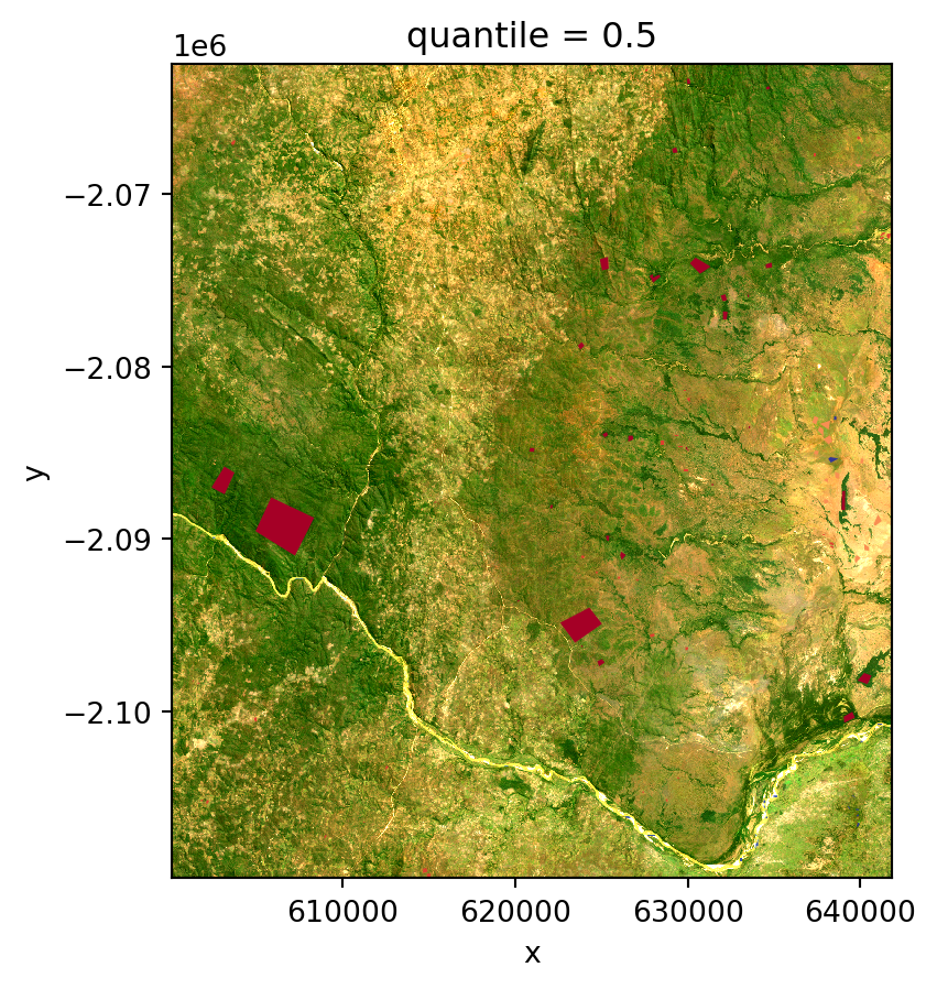
17.2 Prepare Data for Classification
Prior to the actual machine learning classification, the data needs to be preprocessed and organized into a suitable format. The preparation involves several key steps: 1. Rasterization of the polygons to create a mask for the areas of interest. 2. Extraction of pixel values from the image data using the mask. 3. Creation of a feature matrix and target vector for classification from the image data.
# https://rasterio.readthedocs.io/en/stable/api/rasterio.features.html#rasterio.features.rasterize
# Rasterize the polygons
rst: np.ndarray = rasterize(
shapes=slivers.to_crs(crs)[["geometry", "poly_id"]]
.to_records(index=False)
.tolist(),
out_shape=feature_cube["Red"].shape[1:], # only x and y dimensions
transform=affine,
)
# Create a DataArray from the rasterized polygons
label_cube = xr.DataArray(
rst,
coords={"y": feature_cube.y, "x": feature_cube.x},
name="poly_id",
)
# Create a DataFrame from the image data
feature_frame: pd.DataFrame = (
feature_cube.drop_vars("spatial_ref")
.to_dataframe()
.dropna()
.pivot_table(index=["y", "x"], columns="quantile", values=None)
# .unstack(level="quantile")
)
# Rename the columns to include quantile information
def _rename_col(col: tuple[str, float]) -> str:
return f"{col[0]}_P{np.round(100 * col[1], 0).astype(int):03}"
feature_frame.columns = [_rename_col(col) for col in feature_frame.columns]# Create a DataFrame from the label data (originally the polygons)
label_frame: pd.DataFrame = (
label_cube.to_dataframe()
.reset_index()
.merge(slivers[["poly_id", "label"]])
.set_index(["y", "x"])
)
SEED: int = 42
train_frame: pd.DataFrame = (
label_frame.join(feature_frame)
.groupby("poly_id")
.sample(frac=0.7, random_state=SEED)
)
# Prepare the features and target variable for classification
X_train: pd.DataFrame = train_frame.drop(columns=["label", "poly_id"])
y_train: pd.Series = train_frame["label"]
_drop_idx: pd.Index = train_frame.index
y_test: pd.Series = label_frame.join(feature_frame).drop(index=_drop_idx)["label"]17.3 Classify Forest Cover with Scikit-learn
We will proceed with training a Random Forest classifier using the prepared data. This process involves the following key steps: 1. Data Splitting into Training and Testing Sets to evaluate the model’s performance. 2. Model Training on the Training Set. 3. Model Evaluation on the Testing Set. 4. Visualization of Results.
# Classify Forest Cover with Scikit-learn
clf_rf = RandomForestClassifier(
random_state=SEED,
class_weight="balanced",
n_jobs=-1,
)
clf_rf.fit(X=X_train, y=(y_train == LandCoverType.TREE_COVER))RandomForestClassifier(class_weight='balanced', n_jobs=-1, random_state=42)In a Jupyter environment, please rerun this cell to show the HTML representation or trust the notebook.
On GitHub, the HTML representation is unable to render, please try loading this page with nbviewer.org.
Parameters
| n_estimators | 100 | |
| criterion | 'gini' | |
| max_depth | None | |
| min_samples_split | 2 | |
| min_samples_leaf | 1 | |
| min_weight_fraction_leaf | 0.0 | |
| max_features | 'sqrt' | |
| max_leaf_nodes | None | |
| min_impurity_decrease | 0.0 | |
| bootstrap | True | |
| oob_score | False | |
| n_jobs | -1 | |
| random_state | 42 | |
| verbose | 0 | |
| warm_start | False | |
| class_weight | 'balanced' | |
| ccp_alpha | 0.0 | |
| max_samples | None | |
| monotonic_cst | None |
With the trained model, we can now make predictions on the image data. The Random Forest classifier will be used to predict the forest cover for each pixel in the image. For that the image data needs to be prepared in a similar way as the training data, as the model expects essentially a vector of features.
# Predict using the trained model
class_frame = pd.DataFrame(
clf_rf.predict(feature_frame),
index=feature_frame.index,
columns=["RF"],
)
# Recreate the DataArray for the predicted forest cover
predicted_forest = (
class_frame.to_xarray().rio.write_crs(crs).rio.write_transform(affine)
)# Map the predicted forest classification
predicted_forest.where(predicted_forest == 1).hvplot.image(
x="x",
y="y",
tiles=True,
cmap="greens",
crs=crs,
hover=False,
)